Seurat常用函数清单

原文：Seurat Command List

原文发布日期：2023年10月31日

为了演示各函数的效果，这里的案例数据选取了在Seurat细胞分群官方教程中用到的包含了2700个细胞的外周血单核细胞数据（pbmc）。数据可在此链接下载。

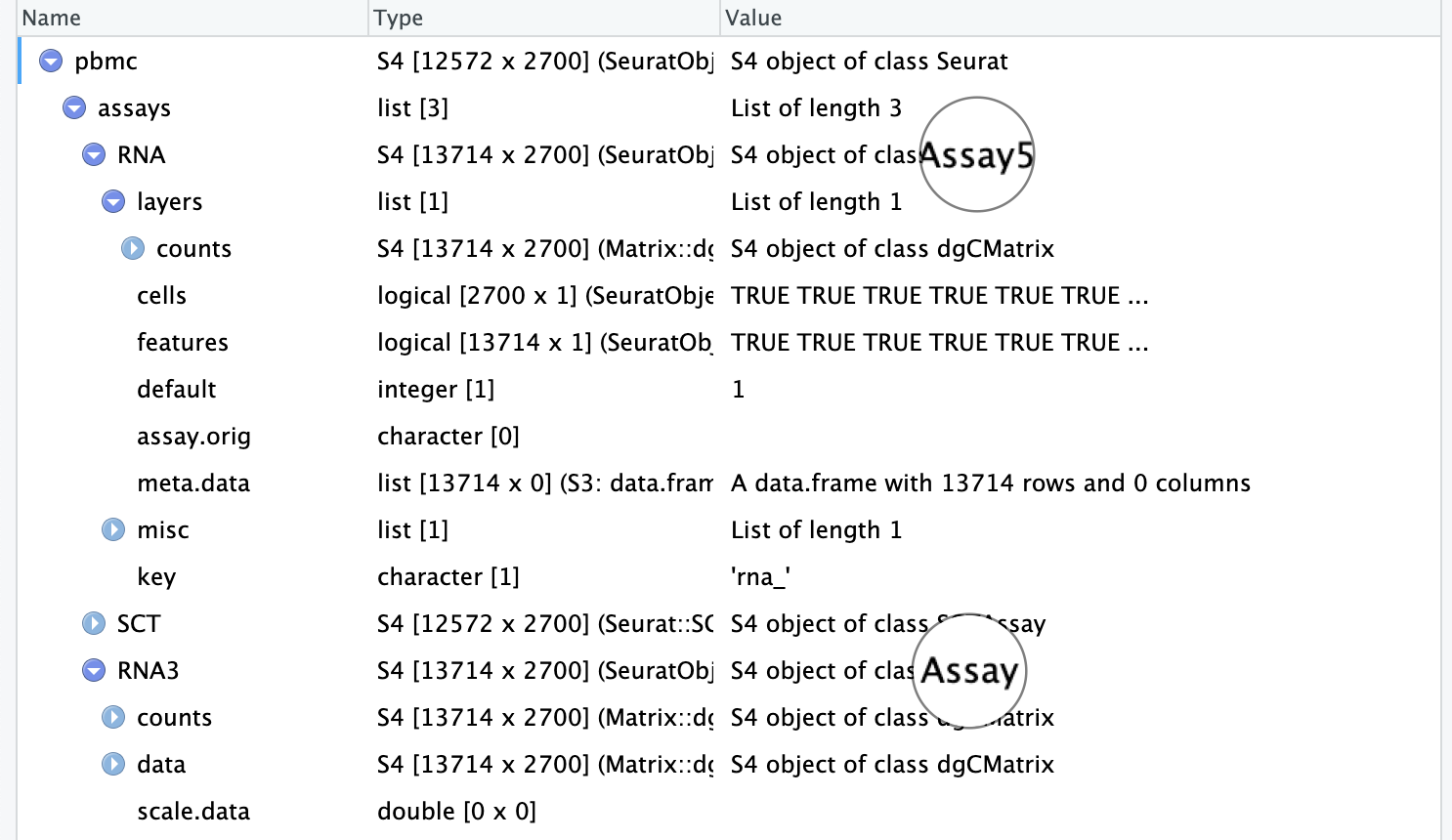
library(Seurat)

# 读取PBMC数据集
counts <- Read10X(data.dir = "data/seurat_official/filtered_gene_bc_matrices/hg19")
# Initialize the Seurat object with the raw (non-normalized data).
pbmc <- CreateSeuratObject(counts = counts, 
                           project = "pbmc3k", 
                           min.cells = 3, 
                           min.features = 200)
pbmc

An object of class Seurat 
13714 features across 2700 samples within 1 assay 
Active assay: RNA (13714 features, 0 variable features)
 1 layer present: counts

---

1 标准Seurat流程基本函数

见Seurat细胞分群官方教程。

pbmc <- NormalizeData(object = pbmc)
pbmc <- FindVariableFeatures(object = pbmc)
pbmc <- ScaleData(object = pbmc)
pbmc <- RunPCA(object = pbmc)
pbmc <- FindNeighbors(object = pbmc, dims = 1:30)
pbmc <- FindClusters(object = pbmc)
pbmc <- RunUMAP(object = pbmc, dims = 1:30)
DimPlot(object = pbmc, reduction = "umap")

1.1 采用SCtransform标准化时的流程：

详见基于SCTransform的单细胞数据标准化。

pbmc <- SCTransform(object = pbmc, verbose = F)
pbmc <- RunPCA(object = pbmc, verbose = F)
pbmc <- FindNeighbors(object = pbmc, dims = 1:30, verbose = F)
pbmc <- FindClusters(object = pbmc, verbose = F)
pbmc <- RunUMAP(object = pbmc, dims = 1:30, verbose = F)
DimPlot(object = pbmc, reduction = "umap")

或者通过管道函数：

pbmc <- SCTransform(pbmc) %>%
    RunPCA() %>%
    FindNeighbors(dims = 1:30) %>%
    FindClusters() %>%
    RunUMAP(dims = 1:30)

---

2 提取Seurat对象内的各数据

2.1 获取细胞、基因、assays、layers名称

获取细胞的barcode：

colnames(pbmc)[1:10]

 [1] "AAACATACAACCAC-1" "AAACATTGAGCTAC-1" "AAACATTGATCAGC-1" "AAACCGTGCTTCCG-1"
 [5] "AAACCGTGTATGCG-1" "AAACGCACTGGTAC-1" "AAACGCTGACCAGT-1" "AAACGCTGGTTCTT-1"
 [9] "AAACGCTGTAGCCA-1" "AAACGCTGTTTCTG-1"

Cells(pbmc)[1:10] # 效果同上

 [1] "AAACATACAACCAC-1" "AAACATTGAGCTAC-1" "AAACATTGATCAGC-1" "AAACCGTGCTTCCG-1"
 [5] "AAACCGTGTATGCG-1" "AAACGCACTGGTAC-1" "AAACGCTGACCAGT-1" "AAACGCTGGTTCTT-1"
 [9] "AAACGCTGTAGCCA-1" "AAACGCTGTTTCTG-1"

获取基因（feature）名。

Features(pbmc)[1:10]

 [1] "AL627309.1"    "RP11-206L10.2" "LINC00115"     "NOC2L"        
 [5] "KLHL17"        "PLEKHN1"       "HES4"          "ISG15"        
 [9] "AGRN"          "C1orf159"     

rownames(pbmc)[1:10] # 同上

 [1] "AL627309.1"    "RP11-206L10.2" "LINC00115"     "NOC2L"        
 [5] "KLHL17"        "PLEKHN1"       "HES4"          "ISG15"        
 [9] "AGRN"          "C1orf159"     

可以指定提取哪一个assay下的基因名，如果未指定，则提取默认assay内的基因名。这里的pbmc数据经过了SCTransform，所以有两个assay，默认的归一化之后的“SCT”assay，另一个是原始的“RNA”assay。

# 获取“SCT” assay下的基因名
Features(pbmc[["SCT"]])[1:10]

 [1] "AL627309.1"    "RP11-206L10.2" "LINC00115"     "NOC2L"        
 [5] "KLHL17"        "PLEKHN1"       "HES4"          "ISG15"        
 [9] "AGRN"          "C1orf159"     

# 获取“RNA” assay下的基因名
Features(pbmc[["RNA"]])[1:10]

 [1] "AL627309.1"    "AP006222.2"    "RP11-206L10.2" "RP11-206L10.9"
 [5] "LINC00115"     "NOC2L"         "KLHL17"        "PLEKHN1"      
 [9] "RP11-54O7.17"  "HES4"         

# 或
Features(pbmc, assay = "RNA")[1:10]

 [1] "AL627309.1"    "AP006222.2"    "RP11-206L10.2" "RP11-206L10.9"
 [5] "LINC00115"     "NOC2L"         "KLHL17"        "PLEKHN1"      
 [9] "RP11-54O7.17"  "HES4"         

也可以通过添加layer参数，提取指定layer下的基因名：

# 提取“counts” layer下的基因名
Features(pbmc, layer = "counts")[1:10]

 [1] "AL627309.1"    "RP11-206L10.2" "LINC00115"     "NOC2L"        
 [5] "KLHL17"        "PLEKHN1"       "HES4"          "ISG15"        
 [9] "AGRN"          "C1orf159"     

# 提取"scale.data"的基因名
Features(pbmc, layer = "scale.data")[1:10]

 [1] "NOC2L"    "HES4"     "ISG15"    "TNFRSF18" "TNFRSF4"  "CPSF3L"  
 [7] "MRPL20"   "ATAD3C"   "SSU72"    "MIB2"    

获取细胞和基因的数量：

ncol(pbmc) # 细胞数量

[1] 2700

nrow(pbmc) # 基因（feature）数量

[1] 12572

获取高变基因列表

详见识别高变基因（highly variable features）。

VariableFeatures(pbmc)[1:10]

 [1] "S100A9" "GNLY"   "LYZ"    "S100A8" "NKG7"   "FTL"    "GZMB"   "IGLL5" 
 [9] "FTH1"   "CCL5"  

列出layers

# 列出所有的layers
Layers(pbmc)

[1] "counts"     "data"       "scale.data"

获取/设定assay：

列出所有的assay，如”RNA” assay、运行SCTransform之后的”SCT” assay。一个Seurat对象可以包括多个assay对象，但是在某个时刻，只有一个assay对象是默认激活的。

实际应用场景见此章节。

# 列出所有的assay
Assays(pbmc)

[1] "RNA" "SCT"

# 获取目前的默认assay名称
DefaultAssay(pbmc)

[1] "SCT"

# 设定默认assay
DefaultAssay(pbmc) <- "RNA"
DefaultAssay(pbmc) <- "SCT"

转换不同版本的Seurat对象：

上面我们使用的pbmc对象使用V5版本的Seurat包创建的，可以通过如下命令查看：

# 查看Seurat对象是用哪个版本的Seurat包创建的
pbmc@version

[1] '5.0.1'

这里我们导入在后续章节中用到的案例数据，这个Seurat对象是使用V4版本的Seurat包创建的。

load(bzfile("data/scRNA-seq_online/additional_data/seurat_integrated.RData.bz2"))
seurat_integrated

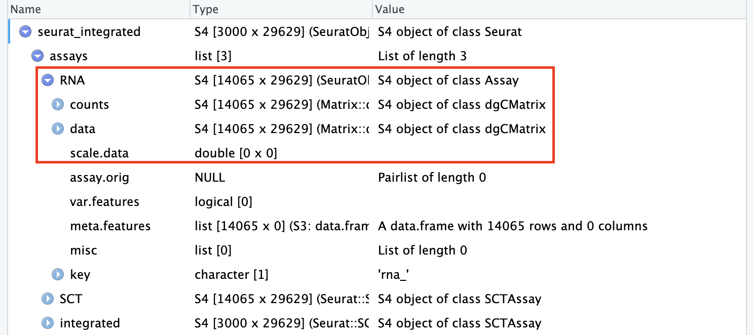
An object of class Seurat 
31130 features across 29629 samples within 3 assays 
Active assay: integrated (3000 features, 3000 variable features)
 2 layers present: data, scale.data
 2 other assays present: RNA, SCT
 2 dimensional reductions calculated: pca, umap

seurat_integrated@version

[1] '4.1.0'

可以看到，这个seurat_integrated对象的“RNA” assay没有layers结构，是典型的V5版本之前的Seurat对象的结构。我们可以通过as()函数将V4或V3版本的“RNA” assay转换成V5版本的“RNA” assay：

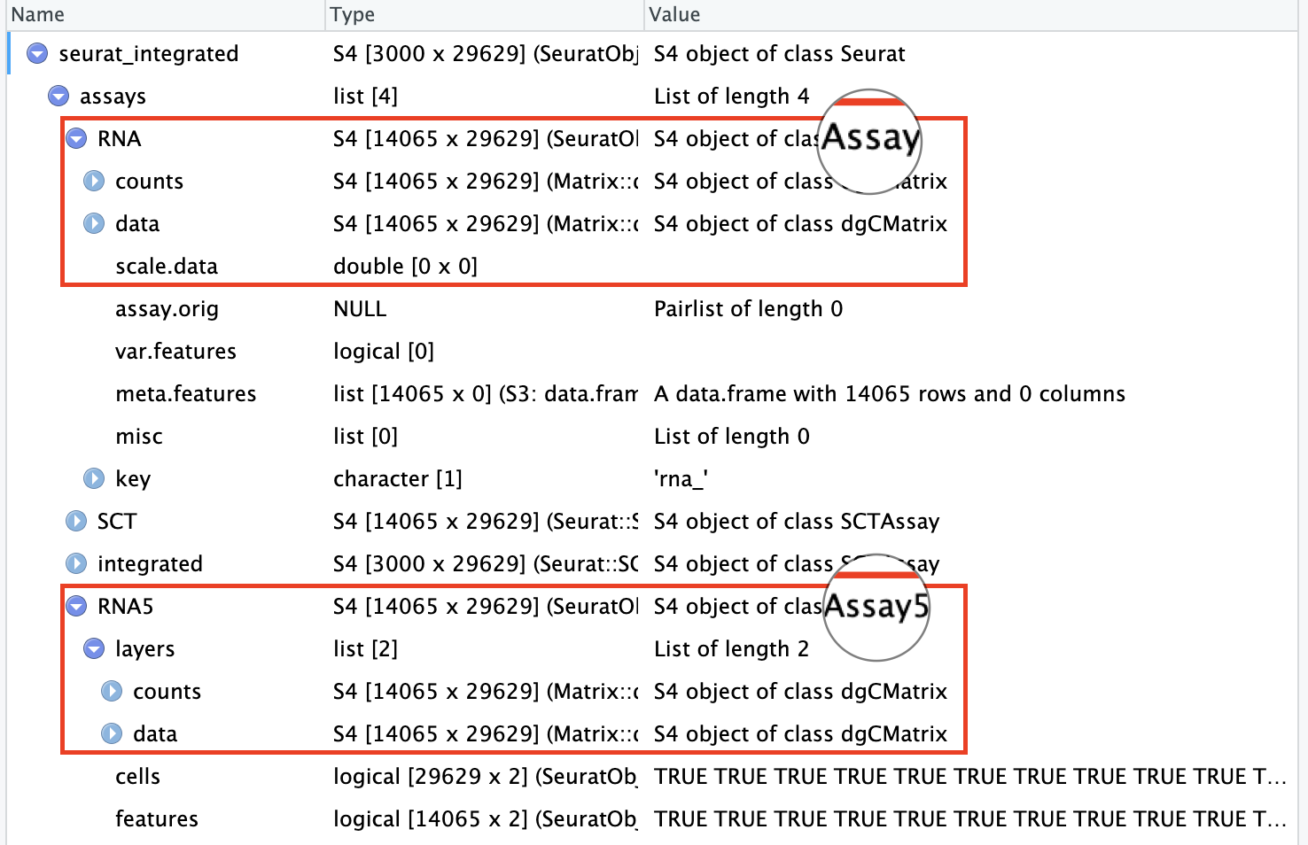
# convert a v4 or v3 assay to a v5 assay
seurat_integrated[["RNA5"]] <- as(object = seurat_integrated[["RNA"]], 
                                  Class = "Assay5")
DefaultAssay(seurat_integrated) = "RNA5"

转换后seurat_integrated[[“RNA5”]]里面是V5版的Seurat结构。如果不想要原来的“RNA” assay可以将其删除：

seurat_integrated[["RNA"]] <- NULL

也可以将V5版本的“RNA” assay转换成V4或V3版本的“RNA” assay：

# convert a v5 assay to a v4 or v3 assay
pbmc[["RNA3"]] <- as(object = pbmc[["RNA"]], Class = "Assay")

2.2 获取细胞注释信息（cell identities）

查看cell identities：

即细胞的类型，在Seurat对象中，细胞可能有好几种不同方法注释的类型，但是在某一时刻，只有一种细胞类型是默认激活的。

Idents(pbmc)[1:5]

AAACATACAACCAC-1 AAACATTGAGCTAC-1 AAACATTGATCAGC-1 AAACCGTGCTTCCG-1 
               4                2                0                5 
AAACCGTGTATGCG-1 
               6 
Levels: 0 1 2 3 4 5 6 7 8 9 10 11 12

table(Idents(pbmc))

  0   1   2   3   4   5   6   7   8   9  10  11  12 
491 485 361 316 229 182 157 153 138 100  42  34  12 

# 查看目前cell identities的水平
levels(pbmc)

 [1] "0"  "1"  "2"  "3"  "4"  "5"  "6"  "7"  "8"  "9"  "10" "11" "12"

设定细胞identities：

实际应用场景见后续章节。

# 将meta.data中的"seurat_clusters"列设置为cell identities
Idents(pbmc) <- "seurat_clusters"

# 重命名细胞注释标签或重新排序细胞类型标签
Idents(pbmc) <- factor(Idents(pbmc), 
                       levels = levels(pbmc),
                       labels = c("pDC", "Mk", "DC", "CD14 Mono", "CD16 Mono", 
                                  "B Activated", "B", "CD8 T", "NK", "T activated", 
                                  "CD4 Naive T", "CD4 Memory T", "epi"))
Idents(pbmc) |> unique()

 [1] CD16 Mono    DC           pDC          B Activated  B           
 [6] CD8 T        Mk           CD14 Mono    T activated  CD4 Naive T 
[11] CD4 Memory T NK           epi         
13 Levels: pDC Mk DC CD14 Mono CD16 Mono B Activated B CD8 T NK ... epi

将目前的cell identities保存到meta.data新的一列中：

# 将目前的cell identities储存到meta.data的"old.ident"列中
pbmc[["old.ident"]] <- Idents(pbmc) 

重命名某个cell identities：

pbmc <- RenameIdents(pbmc, 
                     "B" = "B cell")
Idents(pbmc) |> unique()

 [1] CD16 Mono    DC           pDC          B Activated  B cell      
 [6] CD8 T        Mk           CD14 Mono    T activated  CD4 Naive T 
[11] CD4 Memory T NK           epi         
13 Levels: B cell pDC Mk DC CD14 Mono CD16 Mono B Activated CD8 T ... epi

2.3 获取meta.data

# View metadata data frame, stored in object@meta.data
pbmc@meta.data |> head()

                 orig.ident nCount_RNA nFeature_RNA nCount_SCT nFeature_SCT
AAACATACAACCAC-1     pbmc3k       2419          779       2275          769
AAACATTGAGCTAC-1     pbmc3k       4903         1352       2597         1126
AAACATTGATCAGC-1     pbmc3k       3147         1129       2469         1111
AAACCGTGCTTCCG-1     pbmc3k       2639          960       2343          942
AAACCGTGTATGCG-1     pbmc3k        980          521       1901          551
AAACGCACTGGTAC-1     pbmc3k       2163          781       2148          767
                 SCT_snn_res.0.8 seurat_clusters nCount_RNA3 nFeature_RNA3
AAACATACAACCAC-1               4               4        2419           779
AAACATTGAGCTAC-1               2               2        4903          1352
AAACATTGATCAGC-1               0               0        3147          1129
AAACCGTGCTTCCG-1               5               5        2639           960
AAACCGTGTATGCG-1               6               6         980           521
AAACGCACTGGTAC-1               0               0        2163           781
                   old.ident
AAACATACAACCAC-1   CD16 Mono
AAACATTGAGCTAC-1          DC
AAACATTGATCAGC-1         pDC
AAACCGTGCTTCCG-1 B Activated
AAACCGTGTATGCG-1           B
AAACGCACTGGTAC-1         pDC

# 或
pbmc[[]] |> head()

                 orig.ident nCount_RNA nFeature_RNA nCount_SCT nFeature_SCT
AAACATACAACCAC-1     pbmc3k       2419          779       2275          769
AAACATTGAGCTAC-1     pbmc3k       4903         1352       2597         1126
AAACATTGATCAGC-1     pbmc3k       3147         1129       2469         1111
AAACCGTGCTTCCG-1     pbmc3k       2639          960       2343          942
AAACCGTGTATGCG-1     pbmc3k        980          521       1901          551
AAACGCACTGGTAC-1     pbmc3k       2163          781       2148          767
                 SCT_snn_res.0.8 seurat_clusters nCount_RNA3 nFeature_RNA3
AAACATACAACCAC-1               4               4        2419           779
AAACATTGAGCTAC-1               2               2        4903          1352
AAACATTGATCAGC-1               0               0        3147          1129
AAACCGTGCTTCCG-1               5               5        2639           960
AAACCGTGTATGCG-1               6               6         980           521
AAACGCACTGGTAC-1               0               0        2163           781
                   old.ident
AAACATACAACCAC-1   CD16 Mono
AAACATTGAGCTAC-1          DC
AAACATTGATCAGC-1         pDC
AAACCGTGCTTCCG-1 B Activated
AAACCGTGTATGCG-1           B
AAACGCACTGGTAC-1         pDC

# 如果是展示前6行的话也可以直接这样写：
head(pbmc)

                 orig.ident nCount_RNA nFeature_RNA nCount_SCT nFeature_SCT
AAACATACAACCAC-1     pbmc3k       2419          779       2275          769
AAACATTGAGCTAC-1     pbmc3k       4903         1352       2597         1126
AAACATTGATCAGC-1     pbmc3k       3147         1129       2469         1111
AAACCGTGCTTCCG-1     pbmc3k       2639          960       2343          942
AAACCGTGTATGCG-1     pbmc3k        980          521       1901          551
AAACGCACTGGTAC-1     pbmc3k       2163          781       2148          767
AAACGCTGACCAGT-1     pbmc3k       2175          782       2158          764
AAACGCTGGTTCTT-1     pbmc3k       2260          790       2204          773
AAACGCTGTAGCCA-1     pbmc3k       1275          532       1905          523
AAACGCTGTTTCTG-1     pbmc3k       1103          550       1988          557
                 SCT_snn_res.0.8 seurat_clusters nCount_RNA3 nFeature_RNA3
AAACATACAACCAC-1               4               4        2419           779
AAACATTGAGCTAC-1               2               2        4903          1352
AAACATTGATCAGC-1               0               0        3147          1129
AAACCGTGCTTCCG-1               5               5        2639           960
AAACCGTGTATGCG-1               6               6         980           521
AAACGCACTGGTAC-1               0               0        2163           781
AAACGCTGACCAGT-1               4               4        2175           782
AAACGCTGGTTCTT-1               4               4        2260           790
AAACGCTGTAGCCA-1               4               4        1275           532
AAACGCTGTTTCTG-1               7               7        1103           550
                   old.ident
AAACATACAACCAC-1   CD16 Mono
AAACATTGAGCTAC-1          DC
AAACATTGATCAGC-1         pDC
AAACCGTGCTTCCG-1 B Activated
AAACCGTGTATGCG-1           B
AAACGCACTGGTAC-1         pDC
AAACGCTGACCAGT-1   CD16 Mono
AAACGCTGGTTCTT-1   CD16 Mono
AAACGCTGTAGCCA-1   CD16 Mono
AAACGCTGTTTCTG-1       CD8 T

# Retrieve specific values from the metadata
pbmc$nCount_RNA[1:5]

AAACATACAACCAC-1 AAACATTGAGCTAC-1 AAACATTGATCAGC-1 AAACCGTGCTTCCG-1 
            2419             4903             3147             2639 
AAACCGTGTATGCG-1 
             980 

pbmc[[c("nCount_RNA", "nFeature_RNA")]][1:5,]

                 nCount_RNA nFeature_RNA
AAACATACAACCAC-1       2419          779
AAACATTGAGCTAC-1       4903         1352
AAACATTGATCAGC-1       3147         1129
AAACCGTGCTTCCG-1       2639          960
AAACCGTGTATGCG-1        980          521

# Add metadata, see ?AddMetaData
random_group_labels <- c(rep("Cancer", nrow(pbmc@meta.data)/2), 
                         rep("Control", nrow(pbmc@meta.data)/2))
pbmc$groups <- random_group_labels

2.4 获取表达量信息 (stored as layers in Seurat v5)

# Retrieve data in an expression matrix RNA counts matrix
pbmc[["RNA"]]$counts[1:5, 1:5]

5 x 5 sparse Matrix of class "dgCMatrix"
              AAACATACAACCAC-1 AAACATTGAGCTAC-1 AAACATTGATCAGC-1
AL627309.1                   .                .                .
AP006222.2                   .                .                .
RP11-206L10.2                .                .                .
RP11-206L10.9                .                .                .
LINC00115                    .                .                .
              AAACCGTGCTTCCG-1 AAACCGTGTATGCG-1
AL627309.1                   .                .
AP006222.2                   .                .
RP11-206L10.2                .                .
RP11-206L10.9                .                .
LINC00115                    .                .

# 或
LayerData(pbmc, assay = "RNA", layer = "counts")[1:5, 1:5]

5 x 5 sparse Matrix of class "dgCMatrix"
              AAACATACAACCAC-1 AAACATTGAGCTAC-1 AAACATTGATCAGC-1
AL627309.1                   .                .                .
AP006222.2                   .                .                .
RP11-206L10.2                .                .                .
RP11-206L10.9                .                .                .
LINC00115                    .                .                .
              AAACCGTGCTTCCG-1 AAACCGTGTATGCG-1
AL627309.1                   .                .
AP006222.2                   .                .
RP11-206L10.2                .                .
RP11-206L10.9                .                .
LINC00115                    .                .

# Set expression data assume new.data is a new expression matrix
pbmc[["RNA"]]$counts <- new.data
# 或
LayerData(pbmc, assay = "RNA", layer = "counts") <- new.data

2.5 获取PCA降维信息

实际应用场景见分析主成分（PCs）对细胞分群的影响。

# 获取细胞在所有主成分上的评分（坐标）
Embeddings(pbmc, reduction = "pca")[1:5, 1:5]

                       PC_1       PC_2       PC_3       PC_4        PC_5
AAACATACAACCAC-1 -10.165852   1.087645   5.471643 -0.4546899  0.41257085
AAACATTGAGCTAC-1  -5.814405 -11.244759 -13.092125 -0.4389098  0.05922870
AAACATTGATCAGC-1  -8.565823   1.643337   5.732506  2.4871682  2.55774745
AAACCGTGCTTCCG-1  25.632631  -1.695688  -2.335731  3.8829838  0.02413971
AAACCGTGTATGCG-1  -2.536685  21.282498  -9.103048 -5.1031745 -2.71944035

# 或
pbmc[['pca']]@cell.embeddings[1:5, 1:5]

                       PC_1       PC_2       PC_3       PC_4        PC_5
AAACATACAACCAC-1 -10.165852   1.087645   5.471643 -0.4546899  0.41257085
AAACATTGAGCTAC-1  -5.814405 -11.244759 -13.092125 -0.4389098  0.05922870
AAACATTGATCAGC-1  -8.565823   1.643337   5.732506  2.4871682  2.55774745
AAACCGTGCTTCCG-1  25.632631  -1.695688  -2.335731  3.8829838  0.02413971
AAACCGTGTATGCG-1  -2.536685  21.282498  -9.103048 -5.1031745 -2.71944035

# 获取基因在所有主成分上的评分（坐标）
Loadings(pbmc, reduction = "pca")[1:5, 1:5]

              PC_1         PC_2        PC_3        PC_4         PC_5
S100A9  0.19825859 -0.008571611  0.09650808 -0.28883733 -0.005721886
GNLY   -0.02330150  0.195582622 -0.10436066 -0.06562367 -0.093134754
LYZ     0.23833773 -0.023491803  0.06414334 -0.26984270 -0.010442604
S100A8  0.16884448 -0.007179440  0.09962703 -0.29729996 -0.001143372
NKG7   -0.04601942  0.296816129 -0.13906341 -0.08608150 -0.061192287

# 或
pbmc[["pca"]]@feature.loadings[1:5, 1:5]

              PC_1         PC_2        PC_3        PC_4         PC_5
S100A9  0.19825859 -0.008571611  0.09650808 -0.28883733 -0.005721886
GNLY   -0.02330150  0.195582622 -0.10436066 -0.06562367 -0.093134754
LYZ     0.23833773 -0.023491803  0.06414334 -0.26984270 -0.010442604
S100A8  0.16884448 -0.007179440  0.09962703 -0.29729996 -0.001143372
NKG7   -0.04601942  0.296816129 -0.13906341 -0.08608150 -0.061192287

# 提取PCA信息中的第二主成分，并展示对该主成分影响最大的前5个基因名
print(pbmc[["pca"]], dims = 2, nfeatures = 5)

PC_ 2 
Positive:  NKG7, CCL5, GZMB, GNLY, GZMA 
Negative:  HLA-DRA, CD74, CD79A, HLA-DPB1, HLA-DQA1 

# Create custom dimensional reduction loadings matrix is optional
new_reduction <- CreateDimReducObject(embeddings = new.embeddings, 
                                      loadings = new.loadings, 
                                      key = "custom_pca")
# 或
pbmc[["custom_pca"]] <- new_reduction

2.6 通过FetchData从Seurat对象中获取任意信息

FetchData can access anything from expression matrices, cell embeddings, or metadata use the previously listed commands to access entire matrices。通过FetchData可以提取包括表达量数据、PCA分数以及meta.data内的任何变量并形成一个数据框。实际应用场景见分析主成分（PCs）对细胞分群的影响。

FetchData(object = pbmc, 
          vars = c("PC_1", "nFeature_RNA", "MS4A1"), 
          layer = "counts") |> head()

                       PC_1 nFeature_RNA MS4A1
AAACATACAACCAC-1 -10.165852          779     0
AAACATTGAGCTAC-1  -5.814405         1352     4
AAACATTGATCAGC-1  -8.565823         1129     0
AAACCGTGCTTCCG-1  25.632631          960     0
AAACCGTGTATGCG-1  -2.536685          521     0
AAACGCACTGGTAC-1  -6.559842          781     0

---

3 Seurat对象取子集和合并

3.1 取子集

实际应用见过滤细胞。

# 根据meta data中的信息取子集
subset(x = pbmc, subset = groups == "Cancer")

An object of class Seurat 
40000 features across 1350 samples within 3 assays 
Active assay: SCT (12572 features, 3000 variable features)
 3 layers present: counts, data, scale.data
 2 other assays present: RNA, RNA3
 2 dimensional reductions calculated: pca, umap

# 提取特定cell identities, also see ?SubsetData
subset(x = pbmc, idents = "B cell")

An object of class Seurat 
40000 features across 157 samples within 3 assays 
Active assay: SCT (12572 features, 3000 variable features)
 3 layers present: counts, data, scale.data
 2 other assays present: RNA, RNA3
 2 dimensional reductions calculated: pca, umap

# 反选
subset(x = pbmc, idents = c("CD4 Naive T", "CD8 T"), invert = TRUE)

An object of class Seurat 
40000 features across 2505 samples within 3 assays 
Active assay: SCT (12572 features, 3000 variable features)
 3 layers present: counts, data, scale.data
 2 other assays present: RNA, RNA3
 2 dimensional reductions calculated: pca, umap

# 根据特定gene/feature表达水平取子集
subset(x = pbmc, subset = S100A9 > 1.5)

An object of class Seurat 
40000 features across 519 samples within 3 assays 
Active assay: SCT (12572 features, 3000 variable features)
 3 layers present: counts, data, scale.data
 2 other assays present: RNA, RNA3
 2 dimensional reductions calculated: pca, umap

# 采用多个标准取子集
subset(x = pbmc, subset = S100A9 > 1.5 & PC_1 > 5)

An object of class Seurat 
40000 features across 517 samples within 3 assays 
Active assay: SCT (12572 features, 3000 variable features)
 3 layers present: counts, data, scale.data
 2 other assays present: RNA, RNA3
 2 dimensional reductions calculated: pca, umap

subset(x = pbmc, subset = S100A9 > 1.5, idents = "CD8 T")

An object of class Seurat 
40000 features across 45 samples within 3 assays 
Active assay: SCT (12572 features, 3000 variable features)
 3 layers present: counts, data, scale.data
 2 other assays present: RNA, RNA3
 2 dimensional reductions calculated: pca, umap

# Downsample the number of cells per identity class
subset(x = pbmc, downsample = 100)

An object of class Seurat 
40000 features across 1088 samples within 3 assays 
Active assay: SCT (12572 features, 3000 variable features)
 3 layers present: counts, data, scale.data
 2 other assays present: RNA, RNA3
 2 dimensional reductions calculated: pca, umap

3.2 分割layers

In Seurat v5, users can now split in object directly into different layers keeps expression data in one object, but splits multiple samples into layers can proceed directly to integration workflow after splitting layers。实际应用场景见数据整合。

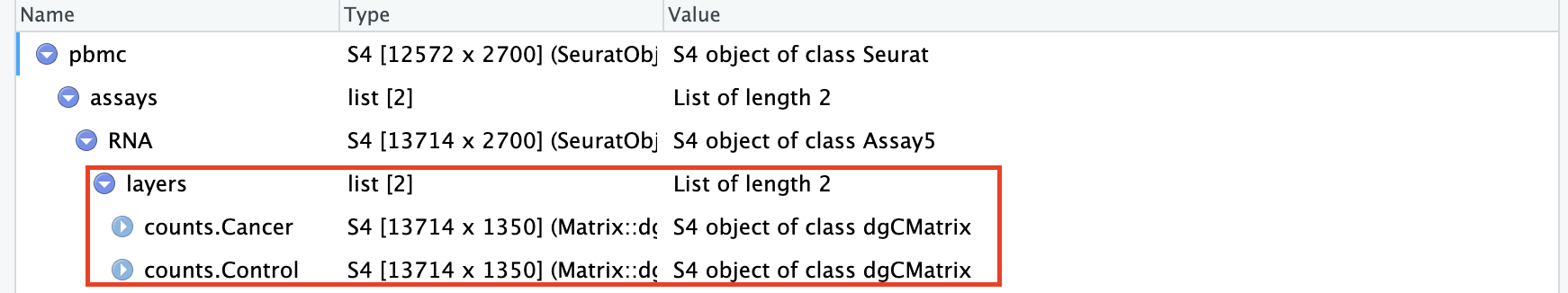
DefaultAssay(pbmc) <- "RNA"
# 按照meta.data中的stim列分割layer
pbmc[["RNA"]] <- split(pbmc[["RNA"]], f = pbmc$groups)

如果需要，例如在整合之后，可以将各layers再次合并在一起：

pbmc[["RNA"]] <- JoinLayers(pbmc[["RNA"]])

3.3 分割Seurat

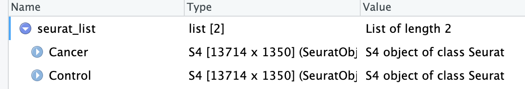
In line with prior workflows, you can also split your Seurat object into a list of multiple objects based on a metadata column creates a list of two objects。通过SplitObject()分割Seurat之后生成的是包含多个Seurat对象的列表。

seurat_list <- SplitObject(pbmc, split.by = "groups")
seurat_list

$Cancer
An object of class Seurat 
40000 features across 1350 samples within 3 assays 
Active assay: RNA (13714 features, 0 variable features)
 1 layer present: counts
 2 other assays present: SCT, RNA3
 2 dimensional reductions calculated: pca, umap

$Control
An object of class Seurat 
40000 features across 1350 samples within 3 assays 
Active assay: RNA (13714 features, 0 variable features)
 1 layer present: counts
 2 other assays present: SCT, RNA3
 2 dimensional reductions calculated: pca, umap

3.4 Merge objects (without integration)

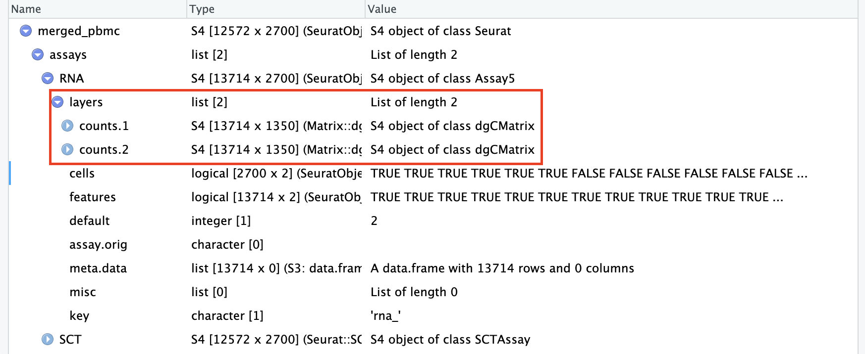
In Seurat v5, merging creates a single object, but keeps the expression information split into different layers for integration. If not proceeding with integration, rejoin the layers after merging. 实际应用场景，见后续章节。

# Merge two Seurat objects
merged_pbmc <- merge(x = seurat_list[["Control"]], 
                     y = seurat_list[["Cancer"]])

# Example to merge more than two Seurat objects
merge(x = pbmc1, 
      y = list(pbmc2, pbmc3))

3.5 Merge objects (with integration)

关于单细胞数据的整合，参考后续章节。

merged_pbmc <- NormalizeData(merged_pbmc, verbose = F)
merged_pbmc <- FindVariableFeatures(merged_pbmc, verbose = F)
merged_pbmc <- ScaleData(merged_pbmc, verbose = F)
merged_pbmc <- RunPCA(merged_pbmc, verbose = F)
merged_pbmc <- IntegrateLayers(object = merged_pbmc, 
                               method = RPCAIntegration, 
                               orig.reduction = "pca", 
                               new.reduction = "integrated.rpca",
                               verbose = FALSE)

# now that integration is complete, rejoin layers
merged_pbmc[["RNA"]] <- JoinLayers(merged_pbmc[["RNA"]])
merged_pbmc

An object of class Seurat 
40000 features across 2700 samples within 3 assays 
Active assay: RNA (13714 features, 2000 variable features)
 3 layers present: data, counts, scale.data
 2 other assays present: SCT, RNA3
 2 dimensional reductions calculated: pca, integrated.rpca

---

Additional resources

Users who are particularly interested in some of the technical changes to data storage in Seurat v5 can explore the following resources:

• SeuratObject manual

• Seurat v5 and Assay5 introductory vignette

---

Session Info

R version 4.3.2 (2023-10-31)
Platform: aarch64-apple-darwin20 (64-bit)
Running under: macOS Sonoma 14.3

Matrix products: default
BLAS:   /Library/Frameworks/R.framework/Versions/4.3-arm64/Resources/lib/libRblas.0.dylib 
LAPACK: /Library/Frameworks/R.framework/Versions/4.3-arm64/Resources/lib/libRlapack.dylib;  LAPACK version 3.11.0

locale:
[1] en_US.UTF-8/en_US.UTF-8/en_US.UTF-8/C/en_US.UTF-8/en_US.UTF-8

time zone: Asia/Shanghai
tzcode source: internal

attached base packages:
[1] stats     graphics  grDevices utils     datasets  methods   base     

other attached packages:
[1] Seurat_5.0.1       SeuratObject_5.0.1 sp_2.1-2          

loaded via a namespace (and not attached):
  [1] RColorBrewer_1.1-3          rstudioapi_0.15.0          
  [3] jsonlite_1.8.8              magrittr_2.0.3             
  [5] spatstat.utils_3.0-4        farver_2.1.1               
  [7] rmarkdown_2.25              zlibbioc_1.48.0            
  [9] vctrs_0.6.5                 ROCR_1.0-11                
 [11] DelayedMatrixStats_1.24.0   spatstat.explore_3.2-5     
 [13] RCurl_1.98-1.14             S4Arrays_1.2.0             
 [15] htmltools_0.5.7             SparseArray_1.2.3          
 [17] sctransform_0.4.1           parallelly_1.36.0          
 [19] KernSmooth_2.23-22          htmlwidgets_1.6.4          
 [21] ica_1.0-3                   plyr_1.8.9                 
 [23] plotly_4.10.4               zoo_1.8-12                 
 [25] igraph_1.6.0                mime_0.12                  
 [27] lifecycle_1.0.4             pkgconfig_2.0.3            
 [29] Matrix_1.6-5                R6_2.5.1                   
 [31] fastmap_1.1.1               GenomeInfoDbData_1.2.11    
 [33] MatrixGenerics_1.14.0       fitdistrplus_1.1-11        
 [35] future_1.33.1               shiny_1.8.0                
 [37] digest_0.6.34               colorspace_2.1-0           
 [39] patchwork_1.2.0             S4Vectors_0.40.2           
 [41] tensor_1.5                  RSpectra_0.16-1            
 [43] irlba_2.3.5.1               GenomicRanges_1.54.1       
 [45] labeling_0.4.3              progressr_0.14.0           
 [47] fansi_1.0.6                 spatstat.sparse_3.0-3      
 [49] httr_1.4.7                  polyclip_1.10-6            
 [51] abind_1.4-5                 compiler_4.3.2             
 [53] withr_3.0.0                 fastDummies_1.7.3          
 [55] R.utils_2.12.3              MASS_7.3-60.0.1            
 [57] DelayedArray_0.28.0         tools_4.3.2                
 [59] lmtest_0.9-40               httpuv_1.6.13              
 [61] future.apply_1.11.1         goftest_1.2-3              
 [63] R.oo_1.25.0                 glmGamPoi_1.14.0           
 [65] glue_1.7.0                  nlme_3.1-164               
 [67] promises_1.2.1              grid_4.3.2                 
 [69] Rtsne_0.17                  cluster_2.1.6              
 [71] reshape2_1.4.4              generics_0.1.3             
 [73] gtable_0.3.4                spatstat.data_3.0-4        
 [75] R.methodsS3_1.8.2           tidyr_1.3.0                
 [77] data.table_1.14.10          XVector_0.42.0             
 [79] utf8_1.2.4                  BiocGenerics_0.48.1        
 [81] spatstat.geom_3.2-7         RcppAnnoy_0.0.21           
 [83] ggrepel_0.9.5               RANN_2.6.1                 
 [85] pillar_1.9.0                stringr_1.5.1              
 [87] spam_2.10-0                 RcppHNSW_0.5.0             
 [89] later_1.3.2                 splines_4.3.2              
 [91] dplyr_1.1.4                 lattice_0.22-5             
 [93] survival_3.5-7              deldir_2.0-2               
 [95] tidyselect_1.2.0            miniUI_0.1.1.1             
 [97] pbapply_1.7-2               knitr_1.45                 
 [99] gridExtra_2.3               IRanges_2.36.0             
[101] SummarizedExperiment_1.32.0 scattermore_1.2            
[103] stats4_4.3.2                xfun_0.41                  
[105] Biobase_2.62.0              matrixStats_1.2.0          
[107] stringi_1.8.3               lazyeval_0.2.2             
[109] yaml_2.3.8                  evaluate_0.23              
[111] codetools_0.2-19            tibble_3.2.1               
[113] cli_3.6.2                   uwot_0.1.16                
[115] xtable_1.8-4                reticulate_1.34.0          
[117] munsell_0.5.0               Rcpp_1.0.12                
[119] GenomeInfoDb_1.38.5         globals_0.16.2             
[121] spatstat.random_3.2-2       png_0.1-8                  
[123] parallel_4.3.2              ellipsis_0.3.2             
[125] ggplot2_3.4.4               dotCall64_1.1-1            
[127] sparseMatrixStats_1.14.0    bitops_1.0-7               
[129] listenv_0.9.0               viridisLite_0.4.2          
[131] scales_1.3.0                ggridges_0.5.5             
[133] crayon_1.5.2                leiden_0.4.3.1             
[135] purrr_1.0.2                 rlang_1.1.3                
[137] cowplot_1.1.2