R version 4.3.2 (2023-10-31)
Platform: aarch64-apple-darwin20 (64-bit)
Running under: macOS Sonoma 14.3
Matrix products: default
BLAS: /Library/Frameworks/R.framework/Versions/4.3-arm64/Resources/lib/libRblas.0.dylib
LAPACK: /Library/Frameworks/R.framework/Versions/4.3-arm64/Resources/lib/libRlapack.dylib; LAPACK version 3.11.0
locale:
[1] en_US.UTF-8/en_US.UTF-8/en_US.UTF-8/C/en_US.UTF-8/en_US.UTF-8
time zone: Asia/Shanghai
tzcode source: internal
attached base packages:
[1] stats graphics grDevices utils datasets methods base
loaded via a namespace (and not attached):
[1] htmlwidgets_1.6.4 compiler_4.3.2 fastmap_1.1.1 cli_3.6.2
[5] tools_4.3.2 htmltools_0.5.7 rstudioapi_0.15.0 yaml_2.3.8
[9] rmarkdown_2.25 knitr_1.45 jsonlite_1.8.8 xfun_0.41
[13] digest_0.6.34 rlang_1.1.3 evaluate_0.23 在Quarto中嵌入Shiny应用程序
Important
本节不涉及Shiny的教程,请在学习本节前确保已基本掌握Shiny的使用,Shiny官方提供了一个很好的Shiny入门指南,通过它可以对Shiny应用程序的开发有一个全局的了解。
本节主要介绍如何在Quarto文档中嵌入Shiny交互式应用程序,而无需依赖服务器。这是一个Quarto的全新特性,感谢Barret Schloerke等人开发的shinylive包让这一特性得以实现。
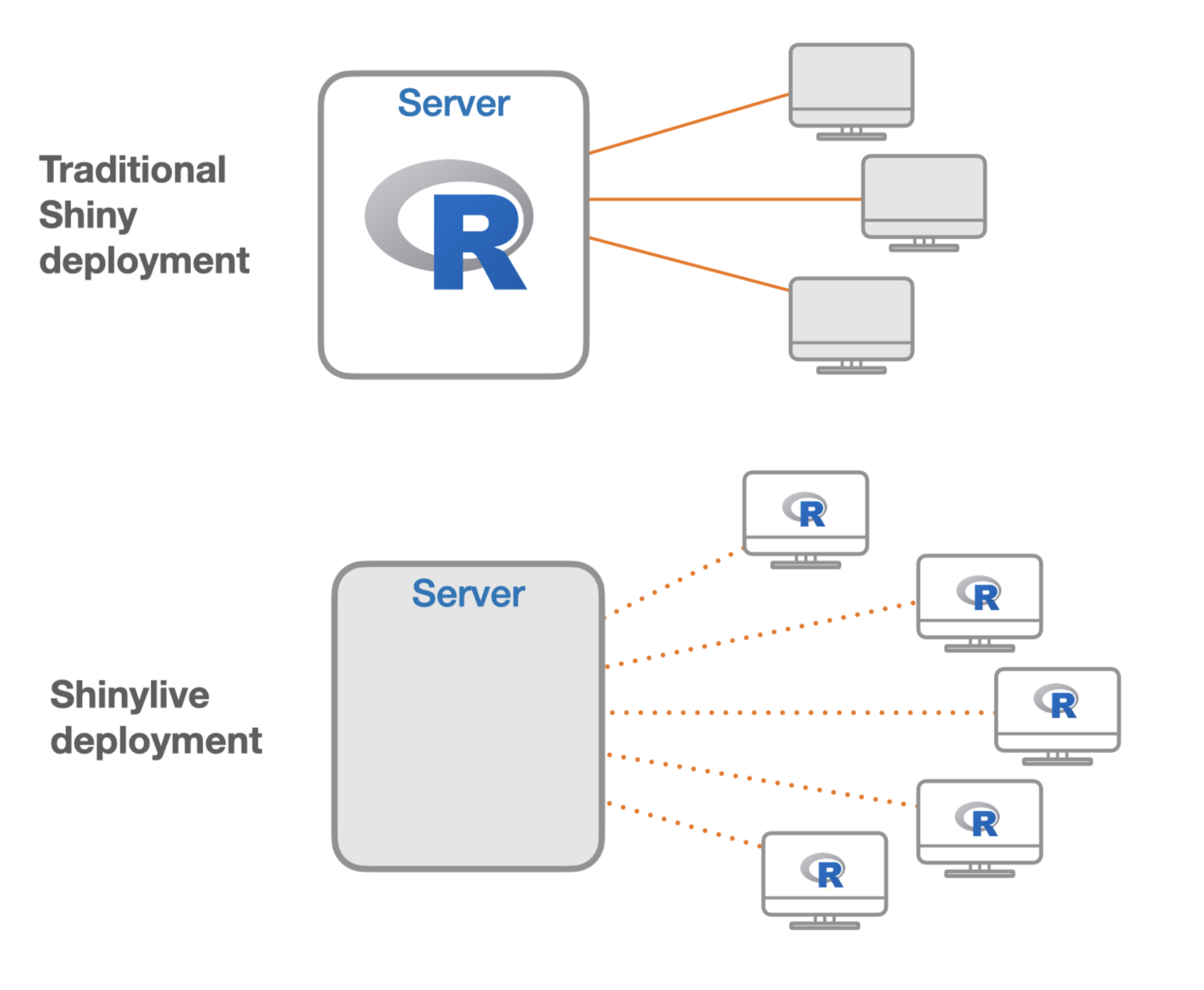
Shinylive是一种非服务器依赖的Shiny,它使得Shiny应用程序能够在网页浏览器中直接运行 ,而不需要依赖后台服务器。在 2022 年的Posit大会上,第一次推出了基于 WebAssembly 和 Pyodide 的 Shinylive for Python。随后,在2023年的Posit大会上,首次推出了基于webR的R版本的shinylive。该包的第一个CRAN版本于2023年10月11日首次发布。
shinylive视频教程《Creating a Serverless R Shiny App using Quarto with R Shinylive》:
Currently, there are three methods (or formats) to use Shinylive applications:
Render a Shiny app into HTML static file using the shinylive package
Host a Shiny app in Fiddle - a built-in web application to run Shiny R and Python applications
Embed Shiny app in Quarto documentation using the quarto-shinylive extension for Quarto (引自:shinylive-r)。
本节我们介绍第三种方法,即在Quarto文档中通过quarto-shinylive extension嵌入Shiny应用程序。
1 安装shinylive包
要实现Shiny应用程序的嵌入,需要依赖shinylive包,可以从CRAN直接安装该包:
install.packages("shinylive")2 建立Quarto Project
创建Quarto项目的方法详见此前的章节。需要注意的是,shinylive 扩展程序必须在 Quarto 项目目录内使用,否则在尝试渲染文档时会报错。错误信息如下:
ERROR:
The shinylive extension must be used in a Quarto project directory
(with a _quarto.yml file).
3 安装shinylive扩展程序
为Quarto安装shinylive扩展程序。在Rstudio终端(Terminal)面板中输入:
quarto add quarto-ext/shinylive
4 YAML设置
为了让Quarto能够调用Shiny应用程序,需要在Quarto文档的YAML设置中加上filters-shinylive命令,如下:
title: "Our first r-shinylive Quarto document!"
filters:
  - shinylive
---
5 编写Shiny程序
我们需要把Shiny程序的代码放到一个特殊的{shinylive-r}代码块内:
```{shinylive-r}
#| standalone: true

library(shiny)

# Define your Shiny UI here
ui <- fluidPage(
  # Your UI components go here
)

# Define your Shiny server logic here
server <- function(input, output, session) {
  # Your server code goes here
}

# Create and launch the Shiny app
shinyApp(ui, server)
```
Caution
{shinylive-r}代码块必须包含 #| standalone: true,这表示代码代表了一个完整的独立 Shiny 应用程序。目前,我们需要把完整的Shiny应用程序的代码,包括ui、server等全部包括进一个代码块内。未来,Quarto可能会支持在一个qmd文档内的多个代码块内分别包含ui、server等结构。
6 渲染Quarto文档
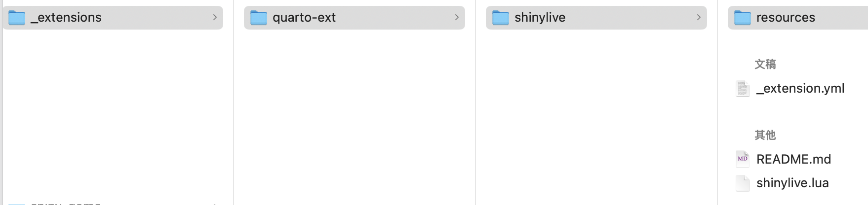
编写好所有内容后,我们即可以通过点击“Render”按钮渲染嵌入了Shiny应用程序的Quarto文档了。渲染后,会在我们的Quarto项目根目录下生成一个_extensions文件夹,其结构如下:
7 发布Quarto文档
一旦制作完成了令人满意的Quarto文档,就可以GitHub Pages和Quarto Pub等通过多种途径发布您的作品了。后面的章节对如何发布GitHub Pages有详细的说明。
Tip
更多关于shinylive的信息,参阅:R-shinylive app in Quarto!
8 案例
8.1 案例一
下面是一个来自Shiny官方入门指南中的案例:
#| standalone: true
#| viewerHeight: 600
library(shiny)

# Define UI ----
ui <- fluidPage(

  # App title ----
  titlePanel("Hello World!"),

  # Sidebar layout with input and output definitions ----
  sidebarLayout(

    # Sidebar panel for inputs ----
    sidebarPanel(

      # Input: Slider for the number of bins ----
      sliderInput(inputId = "bins",
                  label = "Number of bins:",
                  min = 5,
                  max = 50,
                  value = 30)

    ),

    # Main panel for displaying outputs ----
    mainPanel(

      # Output: Histogram ----
      plotOutput(outputId = "distPlot")

    )
  )
)

# Define server logic required to draw a histogram ----
server <- function(input, output) {

  # Histogram of the Old Faithful Geyser Data ----
  # with requested number of bins
  # This expression that generates a histogram is wrapped in a call
  # to renderPlot to indicate that:
  #
  # 1. It is "reactive" and therefore should be automatically
  #    re-executed when inputs (input$bins) change
  # 2. Its output type is a plot
  output$distPlot <- renderPlot({

    x    <- faithful$waiting
    bins <- seq(min(x), max(x), length.out = input$bins + 1)

    hist(x, breaks = bins, col = "#007bc2", border = "orange",
         xlab = "Waiting time to next eruption (in mins)",
         main = "Histogram of waiting times")

    })

}

# Run the app ----
shinyApp(ui = ui, server = server)
代码:
```{shinylive-r}
#| standalone: true
#| viewerHeight: 600
library(shiny)
library(bslib)

# Define UI for app that draws a histogram ----
ui <- page_sidebar(
  sidebar = sidebar(open = "open",
    numericInput("n", "Sample count", 100),
    checkboxInput("pause", "Pause", FALSE),
  ),
  plotOutput("plot", width=1100)
)

server <- function(input, output, session) {
  data <- reactive({
    input$resample
    if (!isTRUE(input$pause)) {
      invalidateLater(1000)
    }
    rnorm(input$n)
  })

  output$plot <- renderPlot({
    hist(data(),
      breaks = 40,
      xlim = c(-2, 2),
      ylim = c(0, 1),
      lty = "blank",
      xlab = "value",
      freq = FALSE,
      main = ""
    )

    x <- seq(from = -2, to = 2, length.out = 500)
    y <- dnorm(x)
    lines(x, y, lwd=1.5)

    lwd <- 5
    abline(v=0, col="red", lwd=lwd, lty=2)
    abline(v=mean(data()), col="blue", lwd=lwd, lty=1)

    legend(legend = c("Normal", "Mean", "Sample mean"),
      col = c("black", "red", "blue"),
      lty = c(1, 2, 1),
      lwd = c(1, lwd, lwd),
      x = 1,
      y = 0.9
    )
  }, res=140)
}

# Create Shiny app ----
shinyApp(ui = ui, server = server)
```
8.2 案例二
#| standalone: true
#| viewerHeight: 500
#| label: fig-shiny-spline

library(ggplot2)
library(htmltools)

ui <- fluidPage(

  fluidRow(
    column(8,
           sliderInput(
             "deg_free",
             label = "Spline degrees of freedom:",
             min = 3L, value = 3L, max = 8L, step = 1L
           )
    ),

    imageOutput("spline_contours", height = "400px")
  )
)


server <- function(input, output, session) {

  # ------------------------------------------------------------------------
  # Input data from remote locations on GitHub

  pred_path <-
    paste(
      "https://raw.githubusercontent.com",
      "topepo", "shinylive-in-book-test",
      "main", "predicted_values.RData",
      sep = "/"
    )
  data_path <-
    paste(
      "https://raw.githubusercontent.com",
      "topepo", "shinylive-in-book-test",
      "main", "sim_val.RData",
      sep = "/"
    )

  rdata_file <- tempfile()
  download.file(pred_path, destfile = rdata_file)
  load(rdata_file)
  download.file(data_path, destfile = rdata_file)
  load(rdata_file)

  # Set some ranges for the plot
  rngs <- list(A = c(-3.3, 3.3), B = c(-4.4, 4.4))

  output$spline_contours <-
    renderImage({

      preds <- predicted_values[predicted_values$deg_free == input$deg_free,]

      p <-
        ggplot(preds, aes(A, B)) +
        # Plot the validation set
        geom_point(
          data = sim_val,
          aes(col = class, pch = class),
          alpha = 1 / 2,
          cex = 3
        ) +
        # Show the class boundary
        geom_contour(
          aes(z = .pred_one),
          breaks = 1 / 2,
          linewidth = 3 / 2,
          col = "black"
        ) +
        # Formatting
        lims(x = rngs$A, y = rngs$B) +
        theme_bw() +
        theme(legend.position = "top")

      file <-
        htmltools::capturePlot(
          print(p),
          tempfile(fileext = ".svg"),
          grDevices::svg,
          width = 4,
          height = 4
        )
      list(src = file)
    },
    deleteFile = TRUE)
}

shinyApp(ui = ui, server = server)
代码:
```{shinylive-r}
#| standalone: true
#| viewerHeight: 500
#| label: fig-shiny-spline

library(ggplot2)
library(htmltools)

ui <- fluidPage(

  fluidRow(
    column(8,
           sliderInput(
             "deg_free",
             label = "Spline degrees of freedom:",
             min = 3L, value = 3L, max = 8L, step = 1L
           )
    ),

    imageOutput("spline_contours", height = "400px")
  )
)


server <- function(input, output, session) {

  # ------------------------------------------------------------------------
  # Input data from remote locations on GitHub

  pred_path <-
    paste(
      "https://raw.githubusercontent.com",
      "topepo", "shinylive-in-book-test",
      "main", "predicted_values.RData",
      sep = "/"
    )
  data_path <-
    paste(
      "https://raw.githubusercontent.com",
      "topepo", "shinylive-in-book-test",
      "main", "sim_val.RData",
      sep = "/"
    )

  rdata_file <- tempfile()
  download.file(pred_path, destfile = rdata_file)
  load(rdata_file)
  download.file(data_path, destfile = rdata_file)
  load(rdata_file)

  # Set some ranges for the plot
  rngs <- list(A = c(-3.3, 3.3), B = c(-4.4, 4.4))

  output$spline_contours <-
    renderImage({

      preds <- predicted_values[predicted_values$deg_free == input$deg_free,]

      p <-
        ggplot(preds, aes(A, B)) +
        # Plot the validation set
        geom_point(
          data = sim_val,
          aes(col = class, pch = class),
          alpha = 1 / 2,
          cex = 3
        ) +
        # Show the class boundary
        geom_contour(
          aes(z = .pred_one),
          breaks = 1 / 2,
          linewidth = 3 / 2,
          col = "black"
        ) +
        # Formatting
        lims(x = rngs$A, y = rngs$B) +
        theme_bw() +
        theme(legend.position = "top")

      file <-
        htmltools::capturePlot(
          print(p),
          tempfile(fileext = ".svg"),
          grDevices::svg,
          width = 4,
          height = 4
        )
      list(src = file)
    },
    deleteFile = TRUE)
}

shinyApp(ui = ui, server = server)
```