Biological heterogeneity in single-cell RNA-seq data is often confounded by technical factors including sequencing depth. The number of molecules detected in each cell can vary significantly between cells, even within the same celltype. Interpretation of scRNA-seq data requires effective pre-processing and normalization to remove this technical variability.
In our manuscript we introduce a modeling framework for the normalization and variance stabilization of molecular count data from scRNA-seq experiments. This procedure omits the need for heuristic steps including pseudocount addition or log-transformation and improves common downstream analytical tasks such as variable gene selection, dimensional reduction, and differential expression. We named this methodsctransform.
Inspired by important and rigorous work from Lause et al (Lause, Berens, and Kobak 2021), we released an updated manuscript (Choudhary and Satija 2022) and updated the sctransform software to a v2 version, which is now the default in Seurat v5.
An object of class Seurat
32738 features across 2700 samples within 1 assay
Active assay: RNA (32738 features, 0 variable features)
 1 layer present: counts
During normalization, we can also remove confounding sources of variation, for example, mitochondrial mapping percentage。SCTransform也可以移除一些非期望变异来源,如线粒体基因的比例。这在传统的单细胞数据分析流程中由ScaleData来完成(见Seurat细胞分群官方教程)。
In Seurat v5, SCT v2 is applied by default. You can revert to v1 by setting vst.flavor = 'v1'
Transformed data will be available in the SCT assay, which is set as the default after running SCTransform:
pbmc[["SCT"]]$scale.data contains the residuals (normalized values), and is used directly as input to PCA. Please note that this matrix is non-sparse, and can therefore take up a lot of memory if stored for all genes. To save memory, we store these values only for variable genes, by setting the return.only.var.genes = TRUE by default in the SCTransform() function call.
To assist with visualization and interpretation, we also convert Pearson residuals back to ‘corrected’ UMI counts. You can interpret these as the UMI counts we would expect to observe if all cells were sequenced to the same depth. If you want to see exactly how we do this, please look at the correct function here.
The ‘corrected’ UMI counts are stored in pbmc[["SCT"]]$counts. We store log-normalized versions of these corrected counts in pbmc[["SCT"]]$data, which are very helpful for visualization.
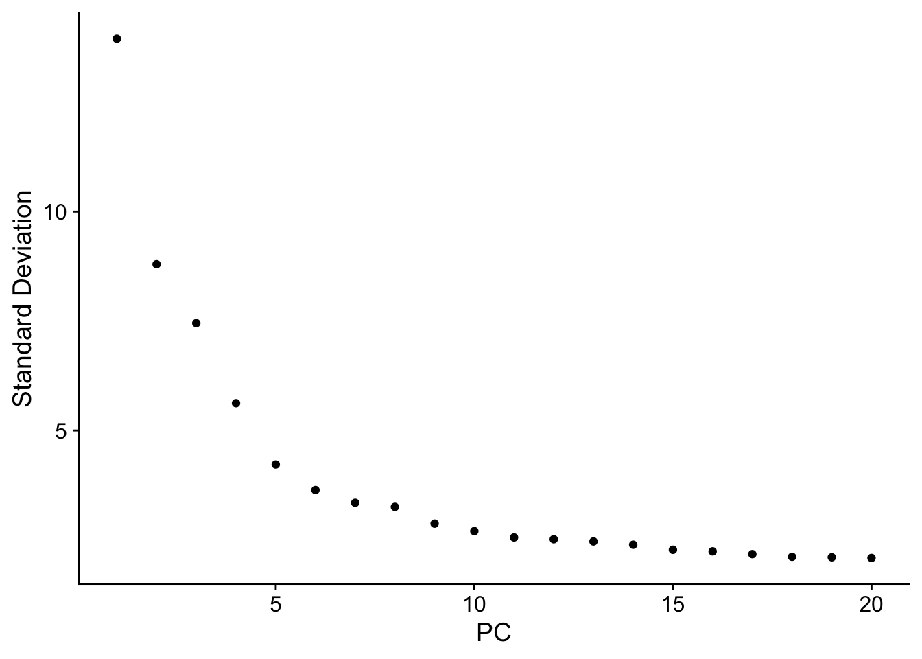
根据Seurat细胞分群官方教程,这个数据集”we can observe an ‘elbow’ around PC9-10, suggesting that the majority of true signal is captured in the first 10 PCs”。因此在FindNeighbors函数中指定了dims = 1:10。但是这里的FindNeighbors函数指定了更多的主成分(dims = 1:30)。下面的内容对此作出了解释:
Why can we choose more PCs when using sctransform?
In the Seurat细胞分群官方教程,we focus on 10 PCs for this dataset, though we highlight that the results are similar with higher settings for this parameter. Interestingly, we’ve found that when using SCTransform, we often benefit by pushing this parameter even higher. We believe this is because the SCTransform workflow performs more effective normalization, strongly removing technical effects from the data.
Even after standard log-normalization, variation in sequencing depth is still a confounding factor (see Figure 1), and this effect can subtly influence higher PCs. In SCTransform, this effect is substantially mitigated (see Figure 3). This means that higher PCs are more likely to represent subtle, but biologically relevant, sources of heterogeneity – so including them may improve downstream analysis.
In addition, SCTransformreturns 3,000 variable features by default, instead of 2,000. The rationale is similar, the additional variable features are less likely to be driven by technical differences across cells, and instead may represent more subtle biological fluctuations. In general, we find that results produced with SCTransform are less dependent on these parameters (indeed, we achieve nearly identical results when using all genes in the transcriptome, though this does reduce computational efficiency). This can help users generate more robust results, and in addition, enables the application of standard analysis pipelines with identical parameter settings that can quickly be applied to new datasets.
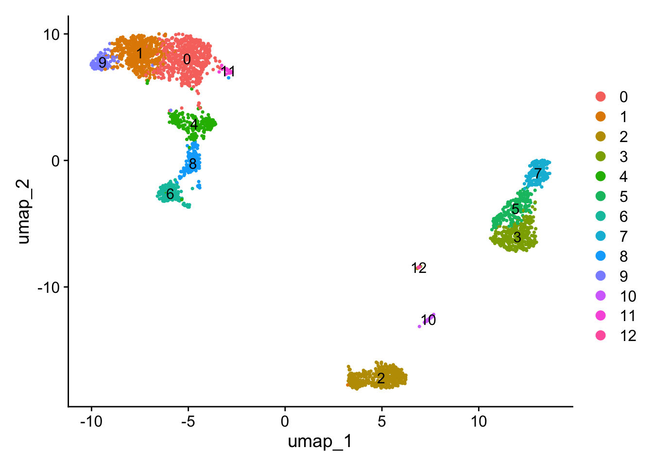
6 Marker基因可视化
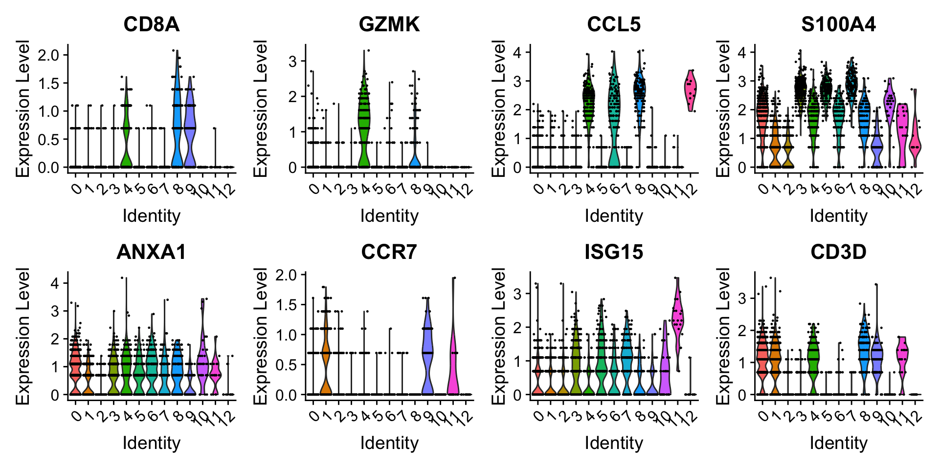
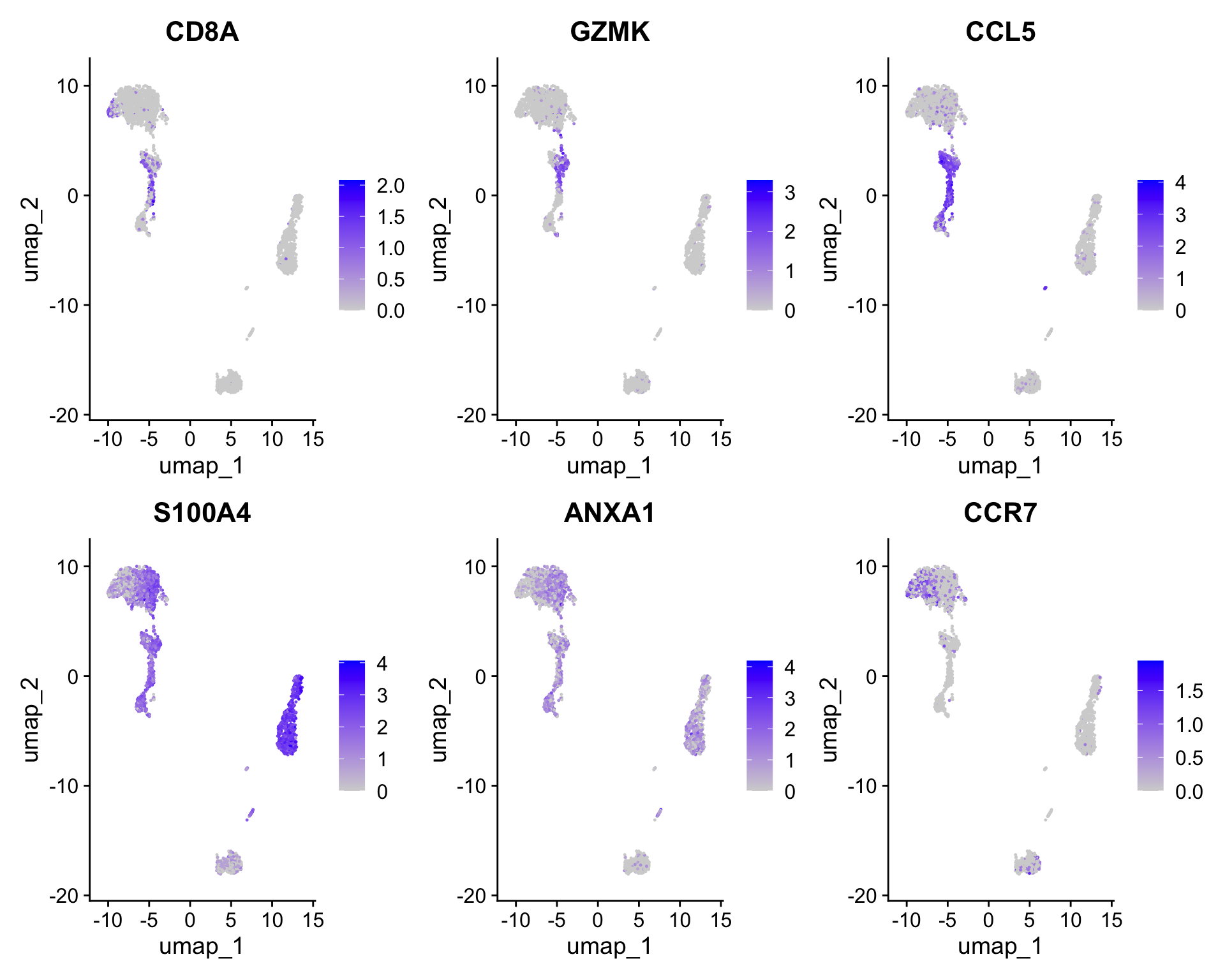
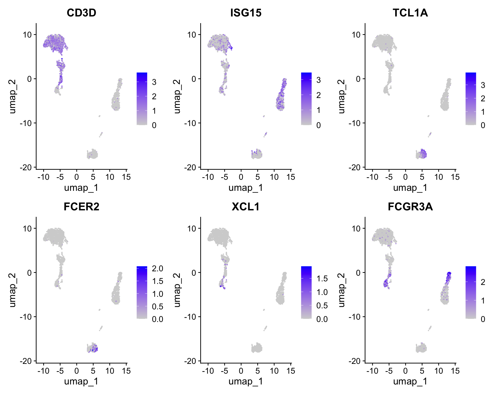
Users can individually annotate clusters based on canonical markers. However, the SCTransform normalization reveals sharper biological distinctions compared to the standard Seurat workflow, in a few ways:
Clear separation of at least 3 CD8 T cell populations (naive, memory, effector), based on CD8A, GZMK, CCL5, CCR7 expression
Clear separation of three CD4 T cell populations (naive, memory, IFN-activated) based on S100A4, CCR7, IL32, and ISG15
Additional developmental sub-structure in B cell cluster, based on TCL1A, FCER2
Additional separation of NK cells into CD56dim vs. bright clusters, based on XCL1 and FCGR3A
Choudhary, Saket, and Rahul Satija. 2022. “Comparison and Evaluation of Statistical Error Models for scRNA-Seq.”Genome Biology 23 (1). https://doi.org/10.1186/s13059-021-02584-9.
Lause, Jan, Philipp Berens, and Dmitry Kobak. 2021. “Analytic Pearson Residuals for Normalization of Single-Cell RNA-Seq UMI Data.”Genome Biology 22 (1). https://doi.org/10.1186/s13059-021-02451-7.
Source Code
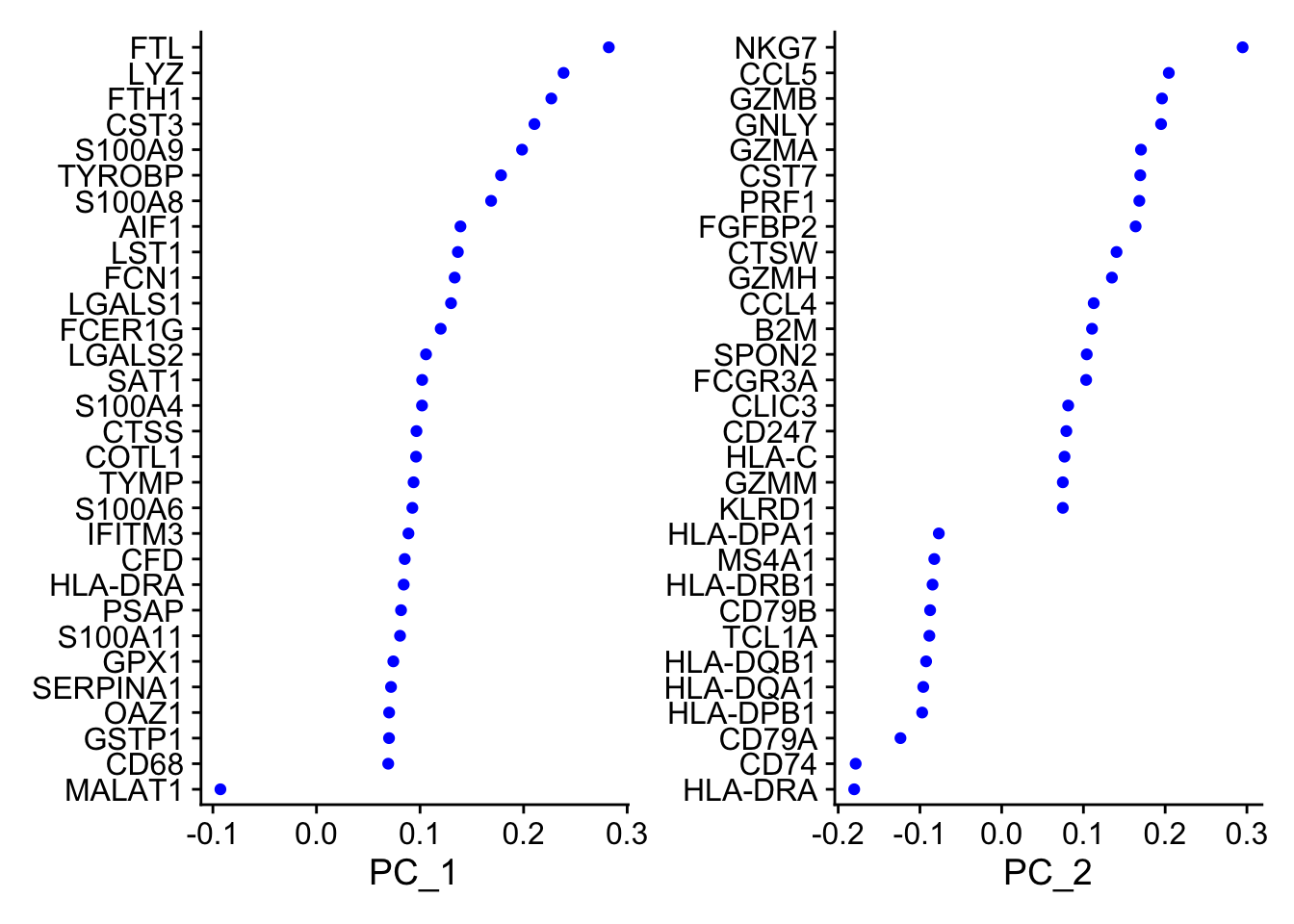
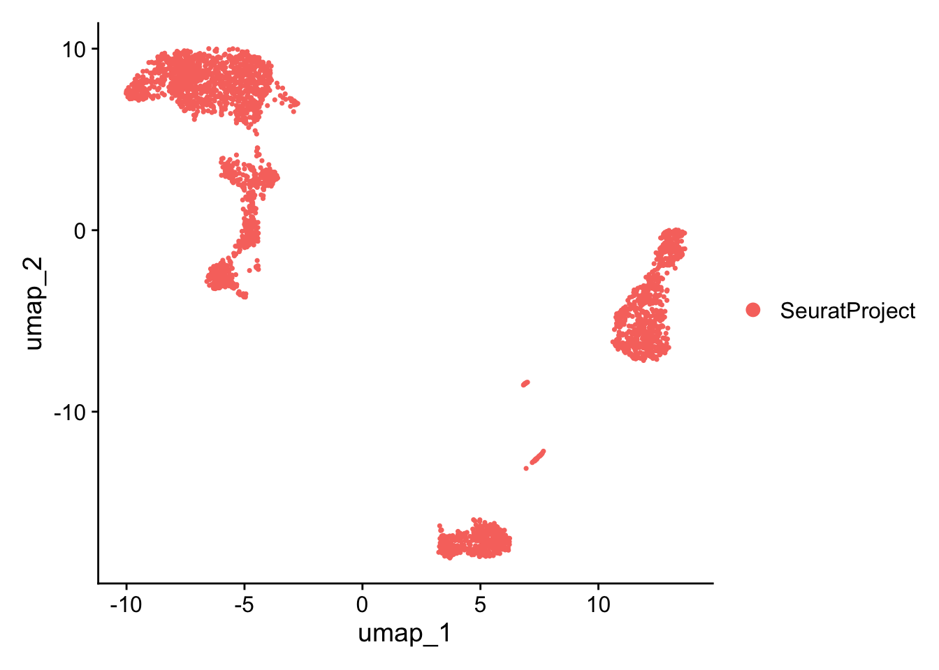
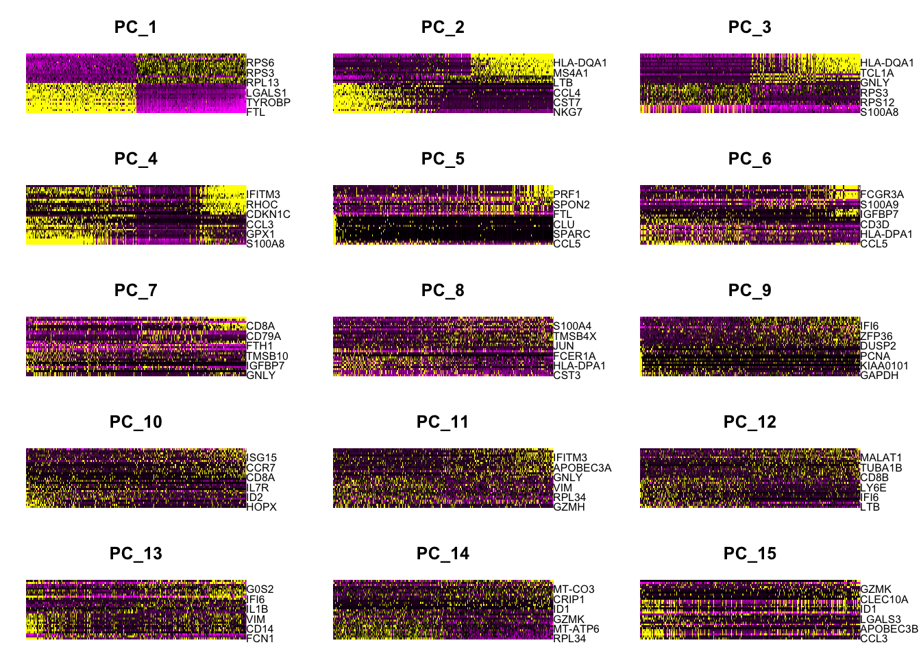
---title: "基于SCTransform的单细胞数据标准化"---> 原文:[*Using sctransform in Seurat*](https://satijalab.org/seurat/articles/sctransform_vignette)>> 原文发布日期:2023年10月31日**Biological heterogeneity** in single-cell RNA-seq data is often confounded by technical factors including **sequencing depth**. The **number of molecules detected in each cell** can vary significantly between cells, even within the same celltype. Interpretation of scRNA-seq data requires effective pre-processing and normalization to remove this **technical variability**.In our manuscript we introduce a modeling framework for the normalization and variance stabilization of molecular count data from scRNA-seq experiments. This procedure **omits the need for heuristic steps** including pseudocount addition or log-transformation and **improves common downstream analytical tasks** such as variable gene selection, dimensional reduction, and differential expression. We named this method`sctransform`.Inspired by important and rigorous work from Lause et al [@lause2021], we released an updated manuscript [@choudhary2022] and updated the sctransform software to a v2 version, which is now the default in Seurat v5.# 载入数据```{r}library(Seurat)pbmc_data <-Read10X(data.dir ="data/seurat_official/filtered_gene_bc_matrices/hg19")pbmc <-CreateSeuratObject(counts = pbmc_data)pbmc```# 质控这里的质控步骤只简单的计算了线粒体基因的比例。```{r}pbmc <-PercentageFeatureSet(pbmc, pattern ="^MT-", col.name ="percent.mt")head(pbmc@meta.data, 5)```# 运行`SCTransform` {#sec-perform_sctransform}- `SCTransform()`替代了传统单细胞数据分析流程中的`NormalizeData()`、`ScaleData()`和`FindVariableFeatures()`函数的功能,因此不再需要运行这些函数。- During normalization, we can also remove confounding sources of variation, for example, mitochondrial mapping percentage。`SCTransform`也可以移除一些非期望变异来源,如线粒体基因的比例。这在传统的单细胞数据分析流程中由`ScaleData`来完成(见[Seurat细胞分群官方教程](/single_cell/seurat/seurat_tutorial.qmd#sec-scaledata))。- In Seurat v5, SCT v2 is applied by default. You can revert to v1 by setting `vst.flavor = 'v1'`- `SCTransform`的运算调用了[`glmGamPoi`](https://bioconductor.org/packages/release/bioc/html/glmGamPoi.html)包以显著提升运算速度。所以事先需要通过BiocManager安装该包。```{r}# BiocManager::install("glmGamPoi")pbmc <-SCTransform(pbmc, vars.to.regress ="percent.mt", verbose =FALSE)```Transformed data will be available in the `SCT assay`, which is set as the default after running `SCTransform`: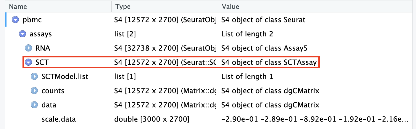- `pbmc[["SCT"]]$scale.data` contains the residuals (normalized values), and is **used directly as input to PCA**. Please note that **this matrix is non-sparse**, and can therefore take up a lot of memory if stored for all genes. **To save memory, we store these values only for variable genes**, by setting the `return.only.var.genes = TRUE` by default in the `SCTransform()` function call.- To assist with visualization and interpretation, we also convert Pearson residuals back to 'corrected' UMI counts. You can interpret these as the UMI counts we would expect to observe if all cells were sequenced to the same depth. If you want to see exactly how we do this, please look at the correct function [here](https://github.com/ChristophH/sctransform/blob/master/R/denoise.R).- The 'corrected' UMI counts are stored in `pbmc[["SCT"]]$counts`. We store log-normalized versions of these corrected counts in `pbmc[["SCT"]]$data`, which are very helpful for visualization.# 降维```{r}pbmc <-RunPCA(pbmc, verbose =FALSE)pbmc <-RunUMAP(pbmc, dims =1:30, verbose =FALSE)```降维可视化:```{r}VizDimLoadings(pbmc, dims =1:2, reduction ="pca")DimPlot(pbmc, reduction ="umap")DimHeatmap(pbmc, dims =1:15, cells =1000, balanced =TRUE)ElbowPlot(pbmc)```# 聚类 {#sec-clustering}```{r}pbmc <-FindNeighbors(pbmc, dims =1:30, verbose =FALSE)pbmc <-FindClusters(pbmc, verbose =FALSE)DimPlot(pbmc, label =TRUE)```根据[Seurat细胞分群官方教程](/single_cell/seurat/seurat_tutorial.qmd#sec-Determine_pcs_for_subsequent_analyses),这个数据集"we can observe an 'elbow' around PC9-10, suggesting that the majority of true signal is captured in the first 10 PCs"。因此在`FindNeighbors`函数中指定了`dims = 1:10`。但是这里的`FindNeighbors`函数指定了更多的主成分(`dims = 1:30`)。下面的内容对此作出了解释:::: {.callout-tip collapse="true"}###### Why can we choose more PCs when using sctransform?In the [Seurat细胞分群官方教程](/single_cell/seurat/seurat_tutorial.qmd#sec-Determine_pcs_for_subsequent_analyses),we focus on **10 PCs** for this dataset, though we highlight that **the results are similar with higher settings for this parameter**. Interestingly, we've found that when using `SCTransform`, we often **benefit by pushing this parameter even higher**. We believe this is because the `SCTransform` workflow performs more effective normalization, strongly removing technical effects from the data.Even after standard log-normalization, variation in sequencing depth is still a confounding factor (see [Figure 1](https://genomebiology.biomedcentral.com/articles/10.1186/s13059-019-1874-1)), and this effect can subtly influence higher PCs. In `SCTransform`, this effect is substantially mitigated (see [Figure 3](https://genomebiology.biomedcentral.com/articles/10.1186/s13059-019-1874-1)). This means that **higher PCs are more likely to represent subtle, but biologically relevant, sources of heterogeneity** -- so including them may improve downstream analysis.In addition, `SCTransform` **returns 3,000 variable features by default, instead of 2,000**. The rationale is similar, the additional variable features are less likely to be driven by technical differences across cells, and instead may represent more subtle biological fluctuations. In general, we find that results produced with `SCTransform` are less dependent on these parameters (indeed, we achieve nearly identical results when using all genes in the transcriptome, though this does reduce computational efficiency). This can help users generate more robust results, and in addition, enables the application of standard analysis pipelines with identical parameter settings that can quickly be applied to new datasets.:::# Marker基因可视化Users can individually annotate clusters based on canonical markers. However, the `SCTransform` normalization reveals **sharper biological distinctions** compared to the [standard Seurat workflow](/single_cell/seurat/seurat_tutorial.qmd#可视化marker基因的表达), in a few ways:- Clear separation of at least **3 CD8 T cell populations (naive, memory, effector)**, based on **CD8A, GZMK, CCL5, CCR7** expression- Clear separation of **three CD4 T cell populations (naive, memory, IFN-activated)** based on **S100A4, CCR7, IL32,** and **ISG15**- Additional developmental sub-structure in B cell cluster, based on TCL1A, FCER2- Additional separation of NK cells into CD56dim vs. bright clusters, based on XCL1 and FCGR3A## 小提琴图:```{r}#| fig-width: 10VlnPlot(pbmc, features =c("CD8A", "GZMK", "CCL5", "S100A4", "ANXA1", "CCR7", "ISG15", "CD3D"),pt.size =0.2, ncol =4)```## UMAP图:```{r}#| fig-height: 8#| fig-width: 10FeaturePlot(pbmc, features =c("CD8A", "GZMK", "CCL5", "S100A4", "ANXA1", "CCR7"), pt.size =0.2,ncol =3)``````{r}#| fig-height: 8#| fig-width: 10FeaturePlot(pbmc, features =c("CD3D", "ISG15", "TCL1A", "FCER2", "XCL1", "FCGR3A"), pt.size =0.2,ncol =3)```------------------------------------------------------------------------::: {.callout-note collapse="true" icon="false"}## Session Info```{r}sessionInfo()```:::# References {.unnumbered}::: {#refs}:::