An object of class Seurat
27359 features across 13999 samples within 2 assays
Active assay: SCT (13306 features, 3000 variable features)
 3 layers present: counts, data, scale.data
 1 other assay present: RNA
 3 dimensional reductions calculated: pca, umap, integrated.dr
如果是基于NormalizeData标准化的单细胞数据,需要使用”RNA” assay进行差异分析(见下面的数据读取和预处理),如果不是,需要通过DefaultAssay(ifnb) <- "RNA"进行设定。Note that the raw and normalized counts are stored in the counts and data layers of RNA assay. By default, the functions for finding markers will use normalized data. 关于FindMarkers为什么要使用”RNA” assay,参阅:https://github.com/hbctraining/scRNA-seq_online/issues/58
1.3 准备差异表达分析所需变量
We create a column in the meta.data slot to hold both the cell type and treatment information and switch the current Idents to that column.
Please note that p-values obtained from this analysis should be interpreted with caution, as these tests treat each cell as an independent replicate, and ignore inherent correlations between cells originating from the same sample. Such analyses have been shown to find a large number of false positive associations, as has been demonstrated by (Squair et al. 2021), (Zimmerman, Espeland, and Langefeld 2021), (Junttila, Smolander, and Elo 2022), and others. As discussed here (Crowell et al. 2020), DE tests across multiple conditions should expressly utilize multiple samples/replicates, and can be performed after aggregating (‘pseudobulking’) cells from the same sample and subpopulation together. Below, we show how pseudobulking can be used to account for such within-sample correlation.
Warning
这里没有使用进行pseudobulking的原因是,本例中“ctrl”和“sim”组都分别只有一个重复:We do not perform this analysis here, as there is a single replicate in the data.
1.5 可视化差异基因表达
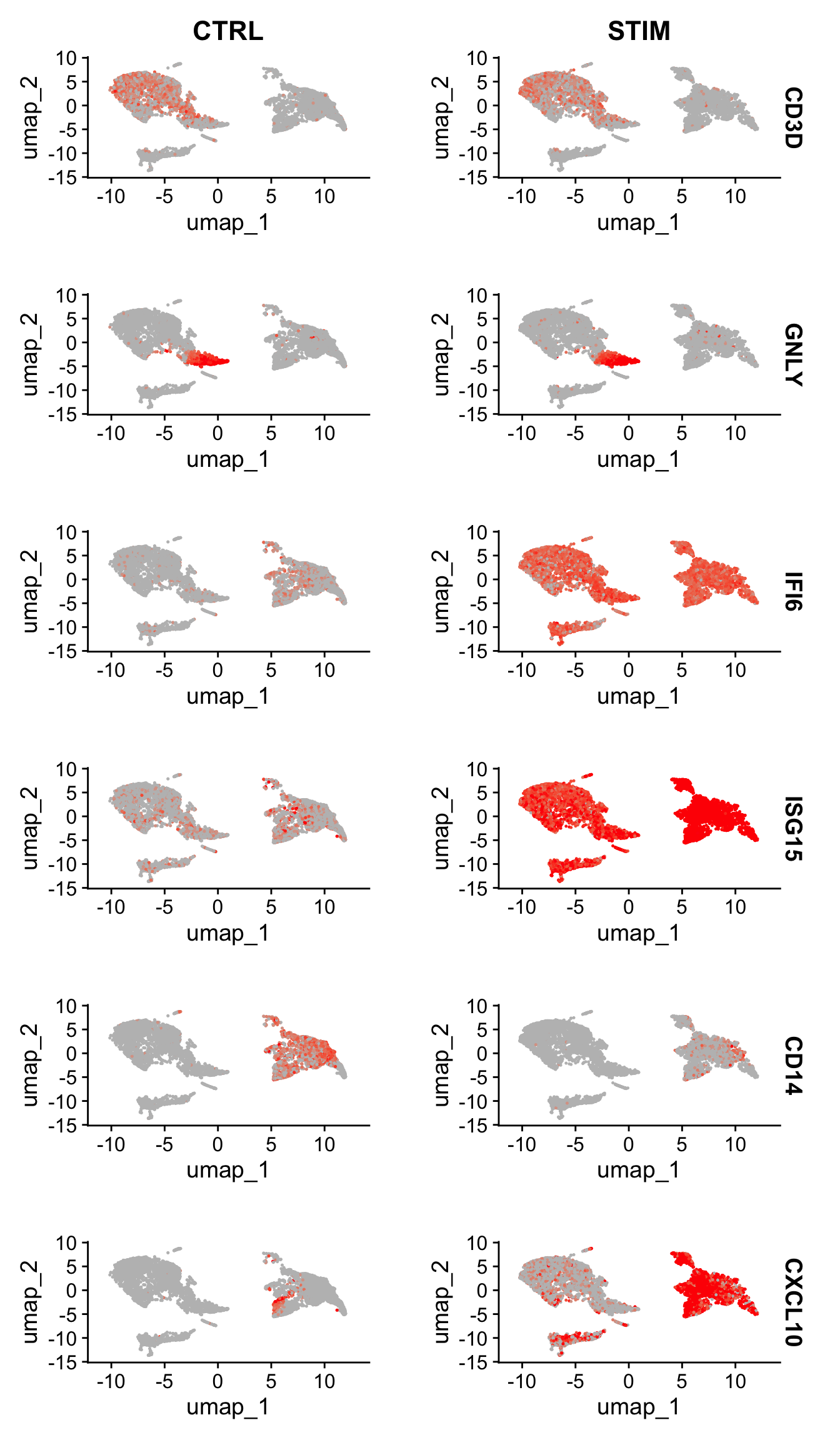
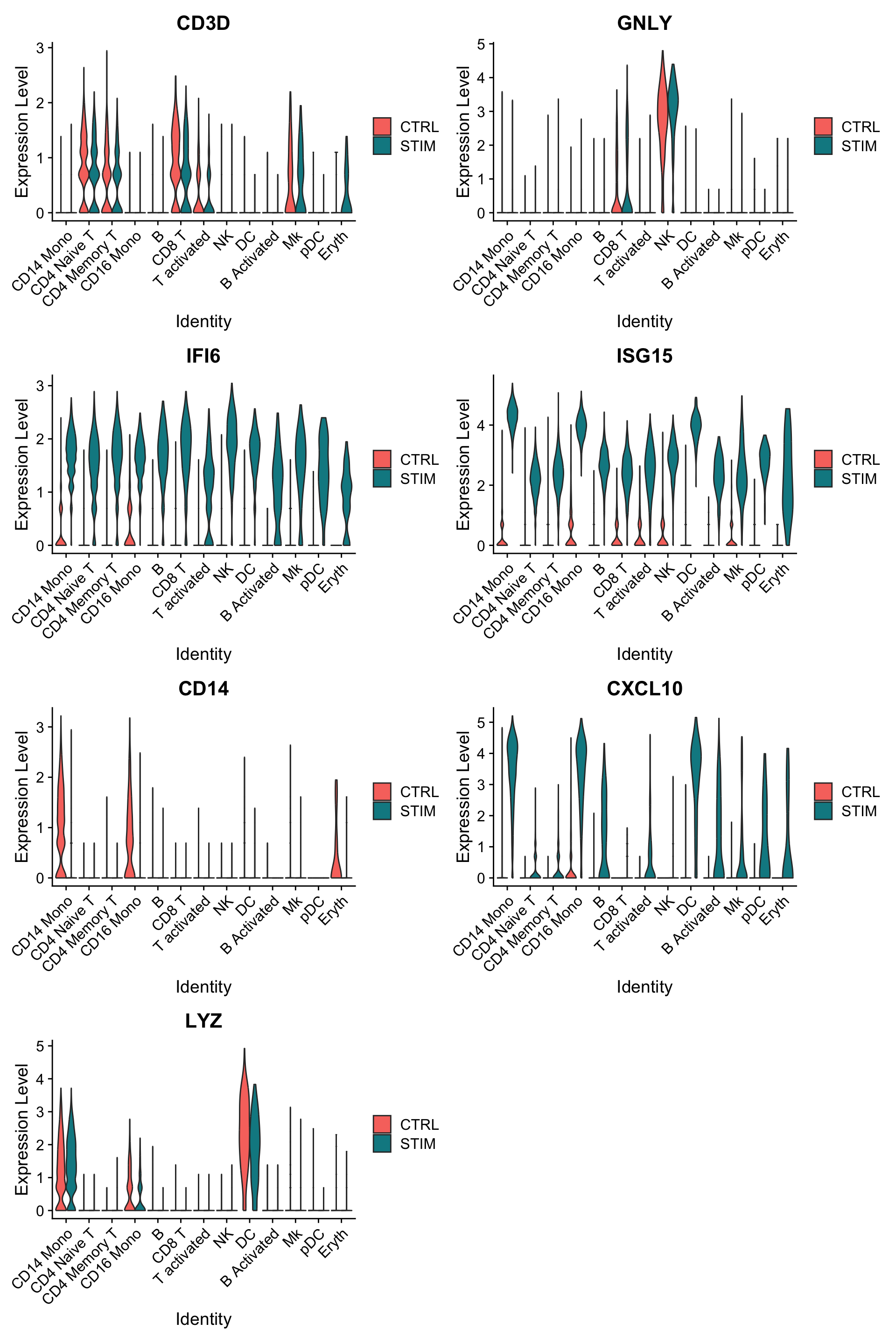
Another useful way to visualize these changes in gene expression is with the split.by option to the FeaturePlot() or VlnPlot() function. This will display FeaturePlots of the list of given genes, split by a grouping variable (stimulation condition here).
Genes such as CD3D and GNLY are canonical cell type markers (for T cells and NK/CD8 T cells) that are virtually unaffected by interferon stimulation and display similar gene expression patterns in the control and stimulated group.
IFI6 and ISG15, on the other hand, are core interferon response genes and are upregulated accordingly in all cell types.
CD14 and CXCL10 are genes that show a cell type specific interferon response.
CD14 expression decreases after stimulation in CD14 monocytes, which could lead to misclassification in a supervised analysis framework, underscoring the value of integrated analysis.如果用于识别细胞类型的marker本身在不同的样本类型(处理 vs. 对照、恶性组织 vs. 正常组织)中存在表达量的差异,那么就会导致对细胞类型判断的错误。而本篇的数据整合则能够避免出现这种情况。
CXCL10 shows a distinct upregulation in monocytes and B cells after interferon stimulation but not in other cell types.
For demonstration purposes, we will be using the interferon-beta stimulated human PBMCs dataset (Kang et al. 2017) that is available via the SeuratData package.
An object of class Seurat
14053 features across 13999 samples within 1 assay
Active assay: RNA (14053 features, 0 variable features)
 2 layers present: counts, data
 [1] CD14 Mono    pDC          CD4 Memory T T activated  CD4 Naive T
 [6] CD8 T        Mk           B Activated  B            DC
[11] CD16 Mono    NK           Eryth
13 Levels: CD14 Mono CD4 Naive T CD4 Memory T CD16 Mono B CD8 T ... Eryth
To pseudobulk, we will use AggregateExpression() to sum together gene counts of all the cells from the same sample for each cell type. This results in one gene expression profile per sampleand cell type. We can then perform DE analysis using DESeq2on the sample level. This treats the samples, rather than the individual cells, as independent observations.
First, we need to retrieve the sample information for each cell. This is not loaded in the metadata, so we will load it from the Github repo of the source data for the original paper.
Add sample information to the dataset
```{r}#| eval: false# 从GitHub仓库读取(可能需要代理)# load the inferred sample IDs of each cellctrl <- read.table(url("https://raw.githubusercontent.com/yelabucsf/demuxlet_paper_code/master/fig3/ye1.ctrl.8.10.sm.best"), head = T, stringsAsFactors = F)stim <- read.table(url("https://raw.githubusercontent.com/yelabucsf/demuxlet_paper_code/master/fig3/ye2.stim.8.10.sm.best"), head = T, stringsAsFactors = F)```
# 可以看到两者的barcode形式不一致# rename the cell IDs by substituting the '-' into '.'info$BARCODE<-gsub(pattern ="\\-", replacement ="\\.", info$BARCODE)info$BARCODE[1:5]
# only keep the cells with high-confidence sample IDinfo<-info[grep(pattern ="SNG", x =info$BEST), ]# remove cells with duplicated IDs in both ctrl and stim groupsinfo<-info[!duplicated(info$BARCODE)&!duplicated(info$BARCODE, fromLast =T), ]# now add the sample IDs to ifnb rownames(info)<-info$BARCODEinfo<-info[, c("BEST"), drop =F]names(info)<-c("donor_id")ifnb<-AddMetaData(ifnb, metadata =info)# remove cells without donor IDsifnb$donor_id[is.na(ifnb$donor_id)]<-"unknown"ifnb<-subset(ifnb, subset =donor_id!="unknown")
按照治疗分组(STIM vs. CTRL)、患者IDs、细胞类型(seurat_annotations)3个条件,执行pseudobulking (AggregateExpression)。通过AggregateExpression命令将同一类型的细胞按照不同的处理条件合并起来,形成一个假的组织水平的测序数据。本例中,有2个治疗分组、13种细胞类型和8个患者,总共被合并成206个类别,将每一个类别看作是一个样本,这样就形成了一个所谓的假的组织水平的测序数据。
An object of class Seurat
14053 features across 206 samples within 1 assay
Active assay: RNA (14053 features, 0 variable features)
 3 layers present: counts, data, scale.data
We also support many other DE tests using other methods. For completeness, the following tests are currently supported:
“wilcox” : Wilcoxon rank sum test (default, using ‘presto’ package)
“wilcox_limma” : Wilcoxon rank sum test (using ‘limma’ package)
“bimod” : Likelihood-ratio test for single cell feature expression, (McDavid et al., Bioinformatics, 2013)
“roc” : Standard AUC classifier
“t” : Student’s t-test
“poisson” : Likelihood ratio test assuming an underlying negative binomial distribution. Use only for UMI-based datasets
“negbinom” : Likelihood ratio test assuming an underlying negative binomial distribution. Use only for UMI-based datasets
“LR” : Uses a logistic regression framework to determine differentially expressed genes. Constructs a logistic regression model predicting group membership based on each feature individually and compares this to a null model with a likelihood ratio test.
“MAST” : GLM-framework that treates cellular detection rate as a covariate (Finak et al, Genome Biology, 2015) (Installation instructions)
“DESeq2” : DE based on a model using the negative binomial distribution (Love et al, Genome Biology, 2014) (Installation instructions) For MAST and DESeq2, please ensure that these packages are installed separately in order to use them as part of Seurat. Once installed, use the test.use parameter can be used to specify which DE test to use.
# Test for DE features using the MAST package# BiocManager::install('limma')Idents(ifnb)<-"seurat_annotations"head(FindMarkers(ifnb, ident.1 ="CD14 Mono", ident.2 ="CD16 Mono", test.use ="wilcox_limma"))
We can see that while the p-values are correlated between the single-cell and pseudobulk data, the single-cell p-values are often smaller and suggest higher levels of significance. In particular, there are 3,519 genes with evidence of differential expression (prior to multiple hypothesis testing) in both analyses, 1,649 genes that only appear to be differentially expressed in the single-cell analysis, and just 204 genes that only appear to be differentially expressed in the bulk analysis.
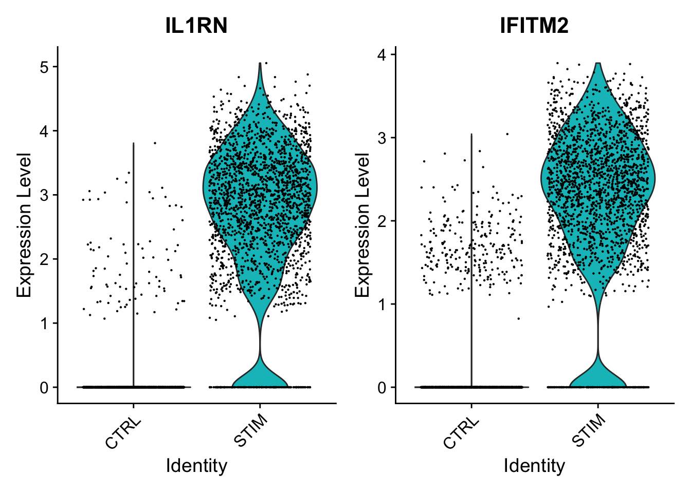
接下来,我们通过小提琴图来检查两种方法中的Top共同差异基因在在刺激组和对照组的表达水平:
# create a new column to annotate sample-condition-celltype in the single-cell datasetifnb$donor_id.stim<-paste0(ifnb$stim, "-", ifnb$donor_id)head(ifnb@meta.data)
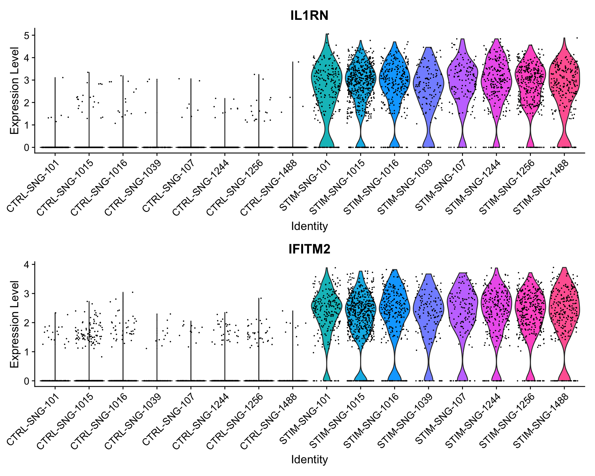
In both the pseudobulk and single-cell analyses, the p-values for these two genes are astronomically small. For both of these genes, when just comparing all stimulated CD4 monocytes to all control CD4 monocytes across samples, we see much higher expression in the stimulated cells.
When breaking down these cells by sample, we continue to see consistently higher expression levels in the stimulated samples compared to the control samples; in other words, this finding is not driven by just one or two samples. Because of this consistency, we find this signal in both analyses.
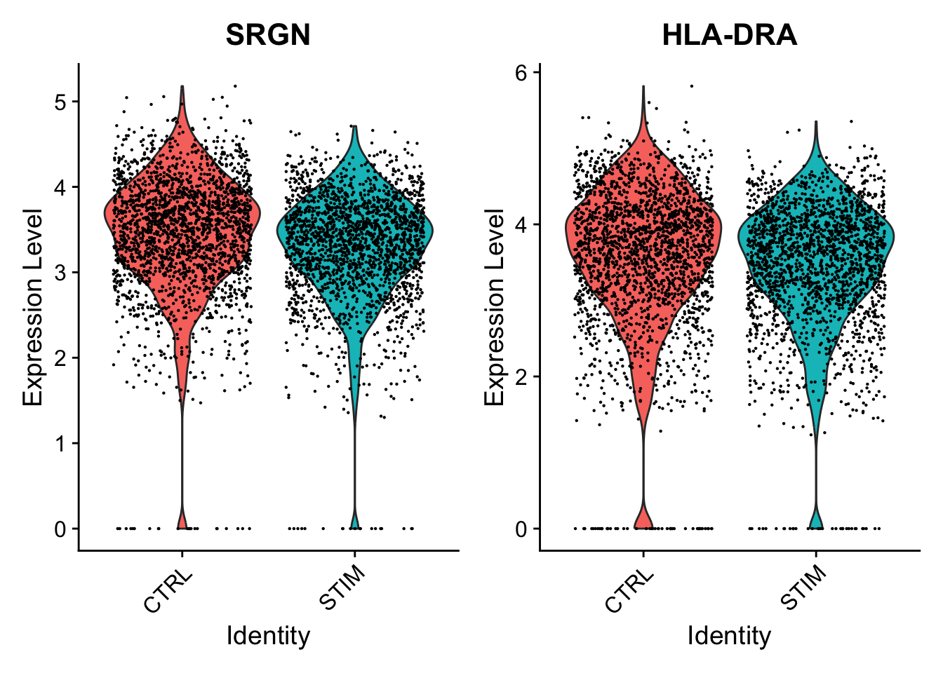
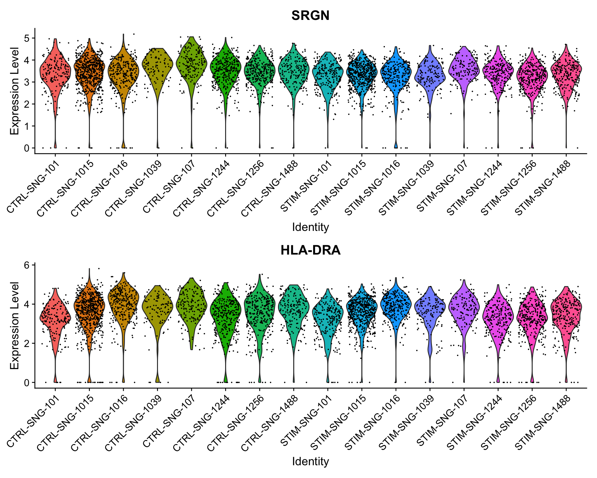
By contrast, we can examine examples of genes that are only DE under the single-cell analysis.
Here, SRGN and HLA-DRA both have very small p-values in the single-cell analysis (on the orders of 10−21 and 10−9), but much larger p-values around 0.18 in the pseudobulk analysis. While there appears to be a difference between control and simulated cells when ignoring sample information, the signal is much weaker on the sample level, and we can see notable variability from sample to sample.
Crowell, Helena L., Charlotte Soneson, Pierre-Luc Germain, Daniela Calini, Ludovic Collin, Catarina Raposo, Dheeraj Malhotra, and Mark D. Robinson. 2020. “Muscat Detects Subpopulation-Specific State Transitions from Multi-Sample Multi-Condition Single-Cell Transcriptomics Data.”Nature Communications 11 (1). https://doi.org/10.1038/s41467-020-19894-4.
Junttila, Sini, Johannes Smolander, and Laura L Elo. 2022. “Benchmarking Methods for Detecting Differential States Between Conditions from Multi-Subject Single-Cell RNA-Seq Data.”Briefings in Bioinformatics 23 (5). https://doi.org/10.1093/bib/bbac286.
Squair, Jordan W., Matthieu Gautier, Claudia Kathe, Mark A. Anderson, Nicholas D. James, Thomas H. Hutson, Rémi Hudelle, et al. 2021. “Confronting False Discoveries in Single-Cell Differential Expression.”Nature Communications 12 (1). https://doi.org/10.1038/s41467-021-25960-2.
Zimmerman, Kip D., Mark A. Espeland, and Carl D. Langefeld. 2021. “A Practical Solution to Pseudoreplication Bias in Single-Cell Studies.”Nature Communications 12 (1). https://doi.org/10.1038/s41467-021-21038-1.
Source Code
---title: "寻找不同样本类型间同一细胞类型内的差异基因"---> 参考原文:[*Introduction to scRNA-seq integration*](https://satijalab.org/seurat/articles/integration_introduction#identify-differential-expressed-genes-across-conditions) *和 [Differential expression testing](https://satijalab.org/seurat/articles/de_vignette)*>> 原文发布日期:2023年10月31日# 直接通过`FindMarkers`寻找差异基因 {#sec-degs_within_the_same_cell_type_between_different_sample_types}## 数据导入导入我们在[整合(integration)](/single_cell/seurat/integration.qmd)中完成`SCTransform`和整合的单细胞数据。这里的meta.data已经提前注释好了细胞类型(储存在"seurat_annotations"列中)。```{r}library(Seurat)ifnb_integrated <-readRDS("output/seurat_official/ifnb_integrated.rds")ifnb_integratedhead(ifnb_integrated, 3)```## 运行`PrepSCTFindMarkers()`,预处理SCT assay```{r}ifnb_integrated <-PrepSCTFindMarkers(ifnb_integrated)```::: callout-important对于经过`SCTransform`归一化处理后的单细胞数据,在进行差异分析之前,需要先运行`PrepSCTFindMarkers()`,来预处理SCT assay。详细解释见[此链接](https://www.jianshu.com/p/fb2e43905559)。如果是基于`NormalizeData`标准化的单细胞数据,需要使用"RNA" assay进行差异分析(见下面的[数据读取和预处理](#数据读取和预处理)),如果不是,需要通过`DefaultAssay(ifnb) <- "RNA"`进行设定。Note that the raw and normalized counts are stored in the `counts` and `data` layers of `RNA` assay. By default, the functions for finding markers will use normalized `data`. 关于`FindMarkers`为什么要使用"RNA" assay,参阅:<https://github.com/hbctraining/scRNA-seq_online/issues/58>:::## 准备差异表达分析所需变量 {#准备差异表达分析所需变量}We create a column in the `meta.data` slot to hold both the cell type and treatment information and switch the current `Idents` to that column.```{r}ifnb_integrated$celltype.stim <-paste(ifnb_integrated$seurat_annotations, ifnb_integrated$stim, sep ="_")unique(ifnb_integrated$celltype.stim)Idents(ifnb_integrated) <-"celltype.stim"```## 执行差异表达分析Then we use `FindMarkers()` to find the genes that are different between control and stimulated B cells.```{r}# 寻找对照组和刺激组之间在B细胞中的差异基因b.interferon.response <-FindMarkers(ifnb_integrated, ident.1 ="B_STIM", ident.2 ="B_CTRL", verbose =FALSE)head(b.interferon.response, n =15)```::: callout-warningPlease note that p-values obtained from this analysis should be interpreted with caution, as **these tests treat each cell as an independent replicate, and ignore inherent correlations between cells originating from the same sample**. Such analyses have been shown to find a large number of **false positive associations**, as has been demonstrated by [@squair2021], [@zimmerman2021], [@junttila2022], and others. As discussed here [@crowell2020], DE tests across multiple conditions should expressly utilize multiple samples/replicates, and can be performed after aggregating (‘pseudobulking’) cells from the same sample and subpopulation together. Below, we show how **pseudobulking** can be used to account for such within-sample correlation.:::::: callout-warning这里没有使用进行pseudobulking的原因是,本例中“ctrl”和“sim”组都分别只有一个重复:We do not perform this analysis here, as there is a single replicate in the data.:::## 可视化差异基因表达Another useful way to visualize these changes in gene expression is with the `split.by` option to the [`FeaturePlot()`](https://satijalab.org/seurat/reference/FeaturePlot.html) or [`VlnPlot()`](https://satijalab.org/seurat/reference/VlnPlot.html) function. This will display FeaturePlots of the list of given genes, split by a grouping variable (stimulation condition here).```{r}#| fig-height: 12FeaturePlot(ifnb_integrated, features =c("CD3D", "GNLY", "IFI6", "ISG15", "CD14", "CXCL10"), split.by ="stim", max.cutoff =3, cols =c("grey", "red"), reduction ="umap")``````{r}#| fig-width: 10#| fig-height: 15plots <-VlnPlot(ifnb_integrated,features =c("CD3D", "GNLY", "IFI6", "ISG15", "CD14", "CXCL10", "LYZ"),split.by ="stim",group.by ="seurat_annotations",pt.size =0,combine =FALSE) # 由于VlnPlot绘制组图时没有图例,所以这里取消绘制组图library(patchwork)wrap_plots(plots = plots, ncol =2) # 将plots列表组合成组图```::: {.callout-note collapse="true"}###### 结果解读- *Genes such as **CD3D** and **GNLY** are canonical cell type markers (for T cells and NK/CD8 T cells) that are virtually **unaffected by interferon stimulation** and **display similar gene expression patterns in the control and stimulated group**.*- ***IFI6** and **ISG15**, on the other hand, are **core interferon response genes** and are **upregulated** accordingly **in all cell types**.*- ***CD14** and **CXCL10** are genes that show a **cell type specific interferon response**.* - ***CD14** expression **decreases** after stimulation in **CD14 monocytes**, [which could lead to misclassification in a supervised analysis framework, underscoring the value of integrated analysis.]{.underline}**如果用于识别细胞类型的marker本身在不同的样本类型(处理 vs. 对照、恶性组织 vs. 正常组织)中存在表达量的差异,那么就会导致对细胞类型判断的错误。而本篇的数据整合则能够避免出现这种情况。*** - ***CXCL10** shows a distinct **upregulation** in **monocytes** and **B cells** after interferon stimulation but not in other cell types.*:::------------------------------------------------------------------------# pseudobulking后的差异分析这一节为了演示pseudobulking,采用的仍然是“ifnb”数据集,仍然包括了“ctrl”和“stim”两个conditions,但是每个条件下都有多个重复,即多个来自不同患者的样本。同时,为了和[Seurat官方教程](https://satijalab.org/seurat/articles/de_vignette)一致,采用了`NormalizeData`对数据进行标准化。## 数据读取和预处理 {#数据读取和预处理}For demonstration purposes, we will be using the interferon-beta stimulated human PBMCs dataset [@kang2017] that is available via the `SeuratData` package.::: {.callout-note collapse="true" appearance="minimal" icon="false"}###### 在线读取(可能需要全局代理)```{r}#| eval: falserm(list =ls())library(Seurat)library(SeuratData)InstallData("ifnb")ifnb <-LoadData("ifnb")```:::从本地下载好的数据读取:```{r}rm(list =ls())library(Seurat)ifnb <-readRDS("data/seurat_official/pbmc_ifnb.rds")ifnbhead(ifnb@meta.data, 5)unique(ifnb$seurat_annotations) # 这里的数据已经提前注释好了细胞类型# 标准化ifnb <-NormalizeData(ifnb)# 核对目前的默认assay,保证是RNA assayDefaultAssay(ifnb)```## 直接通过`FindMarkers`寻找差异基因为了和pseudobulking后的差异分析结果进行比价,这里仍然先进行基于`FindMarkers`的简单差异表达分析,**寻找ctrl和stim之间在CD14单核细胞中的差异基因**。基本步骤和上面的[准备差异表达分析所需变量](#准备差异表达分析所需变量)一致。```{r}ifnb$celltype.stim <-paste(ifnb$seurat_annotations, ifnb$stim, sep ="_")unique(ifnb$celltype.stim)Idents(ifnb) <-"celltype.stim"mono.de <-FindMarkers(ifnb, ident.1 ="CD14 Mono_STIM", ident.2 ="CD14 Mono_CTRL", verbose =FALSE)nrow(mono.de)head(mono.de, n =10)```## 执行pseudobulkingTo pseudobulk, we will use `AggregateExpression()` to sum together **gene counts of all the cells from the same sample** for each cell type. This results in **one gene expression profile per sample** **and cell type**. We can then perform DE analysis using [`DESeq2`](https://bioconductor.org/packages/release/bioc/html/DESeq2.html) **on the sample level**. This treats the samples, rather than the individual cells, as independent observations.First, we need to retrieve the sample information for each cell. This is not loaded in the metadata, so we will load it from the [Github repo](https://github.com/yelabucsf/demuxlet_paper_code/tree/master/) of the source data for the original paper.::: {.callout-tip collapse="true"}###### Add sample information to the dataset```{r}#| eval: false#| echo: fenced# 从GitHub仓库读取(可能需要代理)# load the inferred sample IDs of each cellctrl <-read.table(url("https://raw.githubusercontent.com/yelabucsf/demuxlet_paper_code/master/fig3/ye1.ctrl.8.10.sm.best"), head = T, stringsAsFactors = F)stim <-read.table(url("https://raw.githubusercontent.com/yelabucsf/demuxlet_paper_code/master/fig3/ye2.stim.8.10.sm.best"), head = T, stringsAsFactors = F)``````{r}# 这里提前下载好了两个样本信息文件,所以直接从本地读取ctrl <-readRDS("data/seurat_official/inferred_sample_ids_ctrl.rds")stim <-readRDS("data/seurat_official/inferred_sample_ids_stim.rds")info <-rbind(ctrl, stim)info$BARCODE[1:5]colnames(ifnb)[1:5]# 可以看到两者的barcode形式不一致# rename the cell IDs by substituting the '-' into '.'info$BARCODE <-gsub(pattern ="\\-", replacement ="\\.", info$BARCODE)info$BARCODE[1:5]# only keep the cells with high-confidence sample IDinfo <- info[grep(pattern ="SNG", x = info$BEST), ]# remove cells with duplicated IDs in both ctrl and stim groupsinfo <- info[!duplicated(info$BARCODE) &!duplicated(info$BARCODE, fromLast = T), ]# now add the sample IDs to ifnb rownames(info) <- info$BARCODEinfo <- info[, c("BEST"), drop = F]names(info) <-c("donor_id")ifnb <-AddMetaData(ifnb, metadata = info)# remove cells without donor IDsifnb$donor_id[is.na(ifnb$donor_id)] <-"unknown"ifnb <-subset(ifnb, subset = donor_id !="unknown")```:::可以看到,现在的meta.dat中多了样本信息列(`donor_id`),记录了每个细胞来自哪个患者:```{r}head(ifnb@meta.data, 5)table(ifnb$donor_id, ifnb$stim)```按照治疗分组(STIM vs. CTRL)、患者IDs、细胞类型(seurat_annotations)3个条件,执行pseudobulking (`AggregateExpression`)。通过`AggregateExpression`命令将同一类型的细胞按照不同的处理条件合并起来,形成一个假的组织水平的测序数据。本例中,有2个治疗分组、13种细胞类型和8个患者,总共被合并成206个类别,将每一个类别看作是一个样本,这样就形成了一个所谓的假的组织水平的测序数据。```{r}pseudo_ifnb <-AggregateExpression(ifnb, assays ="RNA", return.seurat = T, group.by =c("stim", "donor_id", "seurat_annotations"))pseudo_ifnbhead(pseudo_ifnb@meta.data) # 可以看到现在的表达矩阵的barcode变成了治疗分组+患者IDs+细胞类型```然后和此前一样,我们在meta.data中增加一列,记录治疗分组(STIM vs. CTRL)+ 细胞类型,这是用于差异分析的分组依据。```{r}pseudo_ifnb$celltype.stim <-paste(pseudo_ifnb$seurat_annotations, pseudo_ifnb$stim, sep ="_")unique(pseudo_ifnb$celltype.stim)```## 执行差异分析 {#sec-perform_de_analysis}Next, we perform DE testing on the pseudobulk level for CD14 monocytes, and compare it against the previous single-cell-level DE results.::: callout-caution###### 安装`DESeq2`包由于pseudobulking后的`FindMarkers`差异分析需要采用`DESeq2`包提供的方法,所以需要提前安装`DESeq2`包:```{r}#| eval: false#| echo: fencedBiocManager::install("DESeq2")```注意,如果是用`FindMarkers`来寻找细胞类型的marker基因,则一般采用默认的Wilcoxon Rank Sum Test方法,这时需要调用的是[`presto`](https://github.com/immunogenomics/presto) 包(见[FindMarkers-在特定cluster之间寻找marker基因](/single_cell/seurat/marker_gene_identification.qmd#sec-findmarkers_function))。:::```{r}Idents(pseudo_ifnb) <-"celltype.stim"bulk.mono.de <-FindMarkers(pseudo_ifnb, ident.1 ="CD14 Mono_STIM", ident.2 ="CD14 Mono_CTRL",test.use ="DESeq2") # 指定差异分析方法为"DESeq2"head(bulk.mono.de, n =15)```::: {.callout-tip collapse="true"}###### `FindMarkers`支持的差异分析方法We also support many other DE tests using other methods. For completeness, the following tests are currently supported:- "wilcox" : Wilcoxon rank sum test (default, using '[presto](https://github.com/immunogenomics/presto)' package)- "wilcox_limma" : Wilcoxon rank sum test (using '[limma](https://bioconductor.org/packages/release/bioc/html/limma.html)' package)- "bimod" : Likelihood-ratio test for single cell feature expression, (McDavid et al., Bioinformatics, 2013)- "roc" : Standard AUC classifier- "t" : Student's t-test- "poisson" : Likelihood ratio test assuming an underlying negative binomial distribution. Use only for UMI-based datasets- "negbinom" : Likelihood ratio test assuming an underlying negative binomial distribution. Use only for UMI-based datasets- "LR" : Uses a logistic regression framework to determine differentially expressed genes. Constructs a logistic regression model predicting group membership based on each feature individually and compares this to a null model with a likelihood ratio test.- "MAST" : GLM-framework that treates cellular detection rate as a covariate (Finak et al, Genome Biology, 2015) (Installation instructions)- "DESeq2" : DE based on a model using the negative binomial distribution (Love et al, Genome Biology, 2014) (Installation instructions) For MAST and DESeq2, please ensure that these packages are installed separately in order to use them as part of Seurat. Once installed, use the test.use parameter can be used to specify which DE test to use.```{r}# Test for DE features using the MAST package# BiocManager::install('limma')Idents(ifnb) <-"seurat_annotations"head(FindMarkers(ifnb, ident.1 ="CD14 Mono", ident.2 ="CD16 Mono", test.use ="wilcox_limma"))```:::------------------------------------------------------------------------## 比较单细胞水平和pseudobulk水平的差异表达分析接下来,我们可以比较一下单细胞水平的差异表达分析的P值和pseudobulk水平的P值:```{r}names(bulk.mono.de) <-paste0(names(bulk.mono.de), ".bulk") # 重命名列bulk.mono.de$gene <-rownames(bulk.mono.de)names(mono.de) <-paste0(names(mono.de), ".sc")mono.de$gene <-rownames(mono.de)merge_dat <-merge(mono.de, bulk.mono.de, by ="gene")merge_dat <- merge_dat[order(merge_dat$p_val.bulk), ]# 查看在两种差异分析方法中P值都有意义的基因名common <- merge_dat$gene[which(merge_dat$p_val.bulk <0.05& merge_dat$p_val.sc <0.05)]# 查看在pseudobulk水平P>0.05但是在单细胞水平P<0.05的基因名:only_sc <- merge_dat$gene[which(merge_dat$p_val.bulk >0.05& merge_dat$p_val.sc <0.05)]# 查看在pseudobulk水平P<0.05但是在单细胞水平P>0.05的基因名:only_bulk <- merge_dat$gene[which(merge_dat$p_val.bulk <0.05& merge_dat$p_val.sc >0.05)]print(paste0('# 在两种差异分析方法中P值都<0.05的基因有: ',length(common), "个"))print(paste0('# 仅在细胞水平差异分析中P值<0.05的基因有: ',length(only_sc), "个"))print(paste0('# 仅在pseudobulk差异分析中P值<0.05的基因有: ',length(only_bulk), "个"))```> We can see that while the p-values are correlated between the single-cell and pseudobulk data, the [**single-cell p-values are often smaller**]{.underline} and suggest higher levels of significance. In particular, there are 3,519 genes with evidence of differential expression (prior to multiple hypothesis testing) in both analyses, 1,649 genes that only appear to be differentially expressed in the single-cell analysis, and just 204 genes that only appear to be differentially expressed in the bulk analysis.接下来,我们通过小提琴图来检查两种方法中的Top共同差异基因在在刺激组和对照组的表达水平:```{r}# create a new column to annotate sample-condition-celltype in the single-cell datasetifnb$donor_id.stim <-paste0(ifnb$stim, "-", ifnb$donor_id)head(ifnb@meta.data)unique(ifnb$celltype.stim)Idents(ifnb) <-"celltype.stim"# 这里我们检查p_val.bulk最小的前两个Top差异基因print(merge_dat[merge_dat$gene %in% common[1:2], c('gene','p_val.sc','p_val.bulk')])# 在细胞类型水平(CD14 Mono)查看这两个Top差异基因在刺激组和对照组的表达水平VlnPlot(ifnb, features = common[1:2], idents =c("CD14 Mono_CTRL", "CD14 Mono_STIM"), group.by ="stim") ``````{r}#| fig-width: 10#| fig-height: 8# 在样本(患者)水平查看这两个Top差异基因在刺激组和对照组的表达水平VlnPlot(ifnb, features = common[1:2], idents =c("CD14 Mono_CTRL", "CD14 Mono_STIM"), group.by ="donor_id.stim", ncol =1) ```> In both the pseudobulk and single-cell analyses, the p-values for these two genes are astronomically small. For both of these genes, when just comparing all stimulated CD4 monocytes to all control CD4 monocytes across samples, we see much higher expression in the stimulated cells.>> When breaking down these cells by sample, we continue to see consistently higher expression levels in the stimulated samples compared to the control samples; in other words, this finding is not driven by just one or two samples. Because of this consistency, we find this signal in both analyses.By contrast, we can examine examples of genes that are only DE under the single-cell analysis.```{r}print(merge_dat[merge_dat$gene %in%c('SRGN','HLA-DRA'), c('gene','p_val.sc','p_val.bulk')])VlnPlot(ifnb, features =c('SRGN','HLA-DRA'), idents =c("CD14 Mono_CTRL", "CD14 Mono_STIM"), group.by ="stim") ``````{r}#| fig-width: 10#| fig-height: 8VlnPlot(ifnb, features =c('SRGN','HLA-DRA'), idents =c("CD14 Mono_CTRL", "CD14 Mono_STIM"), group.by ="donor_id.stim", ncol =1) ```> Here, SRGN and HLA-DRA both have very small p-values in the single-cell analysis (on the orders of 10^−21^ and 10^−9^), but much larger p-values around 0.18 in the pseudobulk analysis. While there appears to be a difference between control and simulated cells when ignoring sample information, the signal is much weaker on the sample level, and we can see notable variability from sample to sample.所以,从这个例子中可以看出**pseudobulk后的差异分析的结果更加准确**。------------------------------------------------------------------------::: {.callout-note collapse="true" icon="false"}## Session Info```{r}#| echo: falsesessionInfo()```:::# References {.unnumbered}::: {#refs}:::