An object of class Seurat
27359 features across 13999 samples within 2 assays
Active assay: SCT (13306 features, 3000 variable features)
 3 layers present: counts, data, scale.data
 1 other assay present: RNA
 3 dimensional reductions calculated: pca, umap, integrated.dr
The results data frame has the following columns :
p_val : p-value (unadjusted)
avg_log2FC : log fold-change of the average expression between the two groups. Positive values indicate that the feature is more highly expressed in the first group.
pct.1 : The percentage of cells where the feature is detected in the first group
pct.2 : The percentage of cells where the feature is detected in the second group
p_val_adj : Adjusted p-value, based on Bonferroni correction using all features in the dataset.
If the ident.2 parameter is omitted or set to NULL, FindMarkers() will test for differentially expressed features between the group specified by ident.1 and all other cells. Additionally, the parameter only.pos can be set to TRUE to only search for positive markers, i.e. features that are more highly expressed in the ident.1 group.
To identify canonical cell type marker genes that are conserved across conditions, we provide the FindConservedMarkers() function. This function performs differential gene expression testing for each dataset/group and combines the p-values using meta-analysis methods from the MetaDE R package.
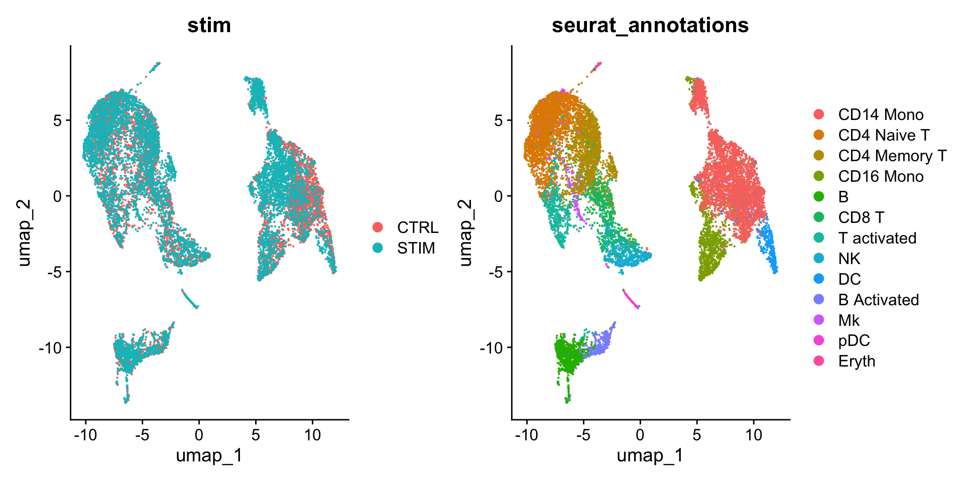
在实际分析中,鉴定这些保守的cell marker主要用来辅助对cluster的注释:you can perform these same analysis on the unsupervised clustering results (stored in seurat_clusters), and use these conserved markers to annotate cell types in your dataset.
We can calculated the genes that are conserved markers irrespective of stimulation condition in cluster 6 (NK cells).
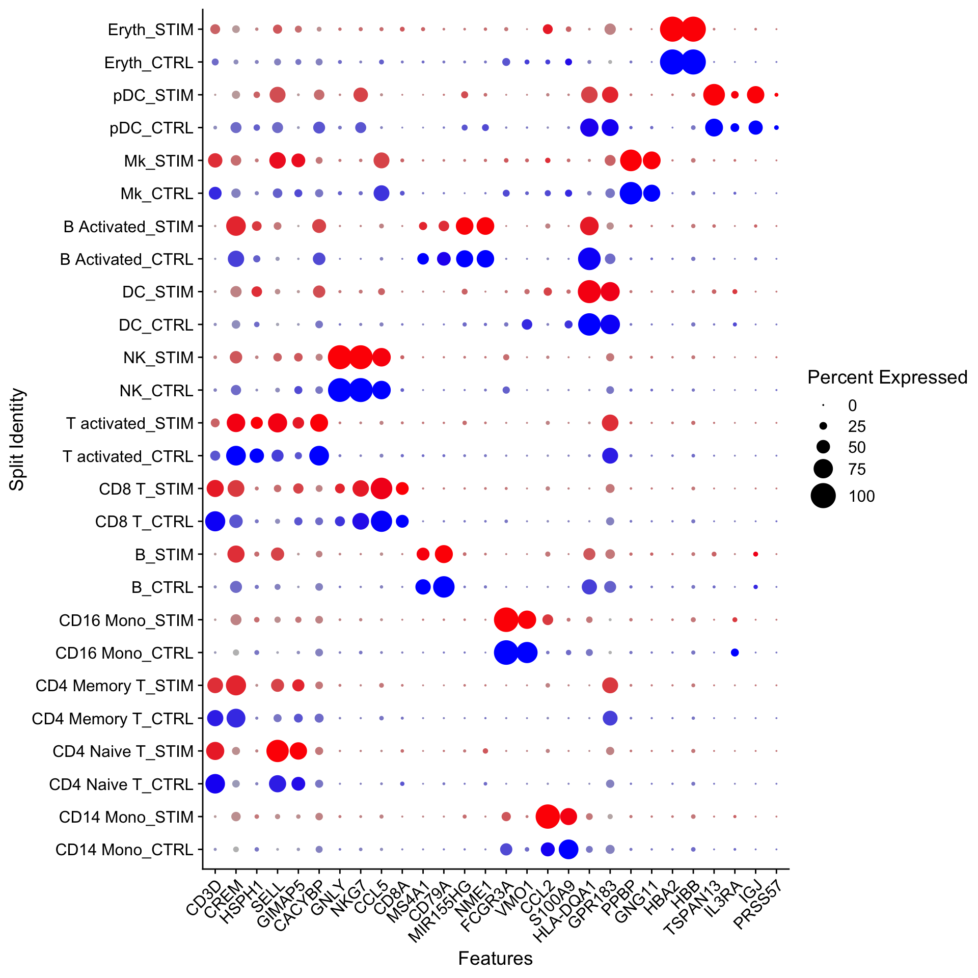
The DotPlot() function with the split.by parameter can be useful for viewing conserved cell type markers across conditions, showing both the expression level and the percentage of cells in a cluster expressing any given gene. Here we plot 2-3 strong marker genes for each of our 14 clusters.
---title: "寻找marker gene"---> 参考原文:[*Introduction to scRNA-seq integration*](https://satijalab.org/seurat/articles/integration_introduction#identify-conserved-cell-type-markers)>> 原文发布日期:2023年10月31日# 数据导入这里我们导入[整合(integration)](/single_cell/seurat/integration.qmd)中完成`SCTransform`和整合的单细胞数据。这里的meta.data已经提前注释好了细胞类型(储存在"seurat_annotations"列中)。```{r}#| fig-width: 10library(Seurat)ifnb <-readRDS("output/seurat_official/ifnb_integrated.rds")ifnbhead(ifnb, 3)table(ifnb$seurat_annotations)DimPlot(ifnb, reduction ="umap", group.by =c("stim", "seurat_annotations"))```# `FindMarkers`-在特定cluster之间寻找marker基因 {#sec-findmarkers_function}::: callout-cautionFor a **much** faster implementation of the Wilcoxon Rank Sum Test,(default method for `FindMarkers`) please install the [`presto`](https://github.com/immunogenomics/presto) package:```{r}#| eval: falsedevtools::install_github('immunogenomics/presto')```:::作为演示,下面我们通过FindMarkers寻找CD16 Mono和CD14 Mono之间的差异基因(marker gene)。::: callout-important对于经过SCTransform归一化处理后的单细胞数据,在进行差异分析之前,需要先运行`PrepSCTFindMarkers()`,来预处理SCT assay。详细解释见[此链接](https://www.jianshu.com/p/fb2e43905559)。如果是基于`NormalizeData`标准化的单细胞数据,需要使用"RNA" assay进行差异分析,如果不是,需要通过`DefaultAssay(ifnb) <- "RNA"`进行设定。:::```{r}# 预处理SCT assayifnb <-PrepSCTFindMarkers(ifnb)# 指定细胞idents为注释信息Idents(ifnb) <-"seurat_annotations"# 执行FindMarkersmonocyte.de.markers <-FindMarkers(ifnb, ident.1 ="CD16 Mono", ident.2 ="CD14 Mono")# view resultsnrow(monocyte.de.markers)head(monocyte.de.markers)```The results data frame has the following columns :- `p_val` : p-value (unadjusted)- `avg_log2FC` : log fold-change of the average expression between the two groups. Positive values indicate that the feature is more highly expressed in the first group.- `pct.1` : The percentage of cells where the feature is detected in the first group- `pct.2` : The percentage of cells where the feature is detected in the second group- `p_val_adj` : Adjusted p-value, based on **Bonferroni correction** using all features in the dataset.If the `ident.2` parameter is omitted or set to `NULL`, `FindMarkers()` will test for differentially expressed features **between the group specified by `ident.1` and all other cells**. Additionally, the parameter `only.pos` can be set to `TRUE` to only search for positive markers, i.e. features that are more highly expressed in the `ident.1` group.```{r}monocyte.de.markers <-FindMarkers(ifnb, ident.1 ="CD16 Mono", ident.2 =NULL, only.pos =TRUE)nrow(monocyte.de.markers)head(monocyte.de.markers)```# FindConservedMarkers-鉴定在所有conditions下保守的cell markerTo **identify canonical cell type marker genes that are conserved across conditions**, we provide the `FindConservedMarkers()` function. This function performs **differential gene expression testing** for each dataset/group and combines the p-values using meta-analysis methods from the `MetaDE` R package.在实际分析中,鉴定这些保守的cell marker主要用来辅助对cluster的注释:you can perform these same analysis on the unsupervised clustering results (stored in `seurat_clusters`), and **use these conserved markers to annotate cell types in your dataset**.We can calculated the genes that are conserved markers irrespective of stimulation condition in cluster 6 (NK cells).::: callout-tip`FindConservedMarkers`函数会调用`metap`包,`metap`包需要`multtest`包,所以需要先安装这两个依赖包:```{r}#| eval: false#| echo: trueBiocManager::install('multtest')install.packages('metap')```:::`FindConservedMarkers`中的`grouping.var`参数用来指定meta.data中表示样本类型或者condition的列名,其他参数及其含义基本和`FindMarkers`一致。```{r}nk.markers <-FindConservedMarkers(ifnb, ident.1 ="NK", grouping.var ="stim", only.pos =TRUE)head(nk.markers)```# 可视化cell markers的表达The `DotPlot()` function with the `split.by` parameter can be useful for viewing conserved cell type markers across conditions, showing both the expression level and the percentage of cells in a cluster expressing any given gene. Here we plot 2-3 strong marker genes for each of our 14 clusters.```{r}#| fig-width: 10#| fig-height: 10markers.to.plot <-c("CD3D", "CREM", "HSPH1", "SELL", "GIMAP5", "CACYBP", "GNLY", "NKG7","CCL5", "CD8A", "MS4A1", "CD79A", "MIR155HG", "NME1", "FCGR3A", "VMO1", "CCL2", "S100A9", "HLA-DQA1", "GPR183", "PPBP", "GNG11","HBA2", "HBB", "TSPAN13", "IL3RA", "IGJ", "PRSS57")DotPlot(ifnb, features = markers.to.plot, cols =c("blue", "red"), dot.scale =8, split.by ="stim") +RotatedAxis()```------------------------------------------------------------------------::: {.callout-note collapse="true" icon="false"}## Session Info```{r}#| echo: falsesessionInfo()```:::